Machine Learning-Based Wine Quality Predictive Modelling

Xiang Li

Metropolitan College, Boston University, One Silber Way, Boston, MA 02215, U.S.A.

Keywords: Wine Quality Prediction, Machine Learning, Random Forest, Oversampling.

Abstract: With the continuous economic development and the trend of consumption upgrading, there is a growing

demand for high-quality wines in the market. Currently, the evaluation of wine quality primarily relies on

scores provided by professional wine tasters. However, leveraging wine physicochemical indicators for

efficient and accurate quality assessment has become increasingly crucial in the industry. In this study, we

utilized a wine dataset sourced from Kaggle to develop and train four machine learning models for predicting

wine quality. To address the issue of imbalanced classes, we incorporated oversampling techniques during

the model training process. Our results demonstrated a significant enhancement in the performance of the

models, with the Random Forest model emerging as the optimal choice. It achieved an accuracy rate of

90.71% for red wine dataset and an impressive accuracy rate of 93.79% for white wine dataset. The findings

of this research underscore the importance of integrating machine learning techniques with wine

physicochemical indicators to enhance the accuracy and efficiency of wine quality assessment.

1 INTRODUCTION

With the development of today’s economy and

society, people’s living standards are constantly

improving, and also their consumption ability is

gradually upgrading. At the same time, more and

more people are beginning to understand and enjoy

wine. According to the statistical data of International

Organization of Vine and Wine (OIV), in 2022,

global wine production reached 25.8 billion liters, 1%

decrease compared to 2021. Overall, global wine

production has remained stable at around 26 billion

liters for 4 consecutive years (Zhang et al., 2022 &

Cheng et al., 2018). Italy, France and Spain accounted

for 51% of global wine production. The estimated

global wine consumption in 2022 is 23.2 billion liters.

The EU’s wine consumption reached 11.1 billion

liters, accounting for 48% of global wine

consumption. The United States remains the world’s

largest consumer of wine, with consumption of 3.4

billion liters.

Normally, the evaluation of wine quality is based on

scores obtained from professional wine tasters.

However, there may inevitably be some differences

due to personal expertise and preferences (Zhang et

al., 2022). Moreover, this evaluation method cannot

be applied in the actual production process due to

large quantities of wine. The physicochemical

indicators of wine are also important components for

quality evaluation besides sensory tests. It is difficult

to accurately classify wine due to complicated and

vague relationship between physicochemical and

sensory analysis. So, establishing an effective wine

quality prediction model that can complete the

evaluation of wine quality more efficient, objective

and accurate becomes a requirement.

The purpose of this paper is to apply multiple

machine learning models on readily accessible

analytical data from Kaggle and select the optimal

model to predict wine quality.

2 RELATED WORKS

Regarding the quality evaluation of wine, Zairan

Cheng et al. used Principal Component Analysis

(PCA) to classify wine grapes and verified the

feasibility of the evaluation using multiple regression

analysis (Cheng et al., 2018). Yanyun Yao et al. used

LASSO regression to evaluate wine and reduced the

cost of evaluation and test (Yao et al., 2016).

Paulo Cortez et al. modelled wine preferences

based on physicochemical indicators of wine using

Support Vector Machine, multiple regression and

Neural Networks (Cortez et al., 2009). Mingze Xia et

al. used SVM model to predict wine quality based on

Li, X.

Machine Learning-Based Wine Quality Predictive Modelling.

DOI: 10.5220/0012998000004601

Paper published under CC license (CC BY-NC-ND 4.0)

In Proceedings of the 1st International Conference on Innovations in Applied Mathematics, Physics and Astronomy (IAMPA 2024), pages 86-92

ISBN: 978-989-758-722-1

the physicochemical indicators of wine Xia et al.,

2020). In their study, 3 different kernel functions,

linear, RBF and polynomial, were applied in the SVM

model. And the prediction accuracy of RBF kernel

function was the best. But there’re also some

limitations of SVM. Firstly, the number of possible

kernels is infinite, and it may be hard to choose the

right one. And it can be computationally intensive

when training the model, especially when large

amount of data.

Feng Zhao et al. optimized the learning rate,

weights and thresholds of Neural Networks and

established a Backpropagation Neural Network

prediction model based on adaptive genetic algorithm

optimization for wine quality prediction (Zhao and

Jiang, 2021). The initial weights and thresholds of the

NN are randomly generated, which can cause it to fall

into the local optimum and affect the model training.

Due to the excessive physicochemical indicators of

wine, Wenbing Sun used genetic algorithm to filter

physicochemical indicators and optimized the

weights and thresholds of the Neural Networks to

reduce the time of model training and improve the

generalization ability of the model (Sun, 2017).

Although NN have spurred innovation within the

field of artificial intelligence, there’re some

limitations when applying this method. Firstly,

Neural Networks have “black box” nature. We don’t

know how or why the NN came up with a certain

output. Secondly, NN may take a long time and more

resources to develop and train. In other words, NN are

computationally expensive.

3 METHODS

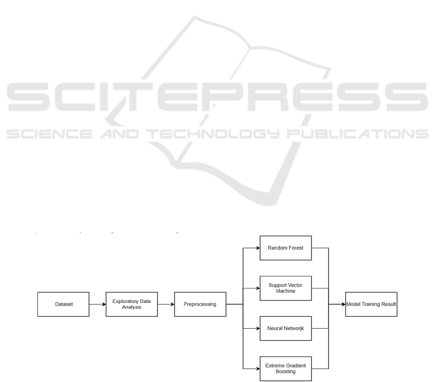
Firstly, we performed exploratory data analysis

(visualization) on the red and white wine dataset

separately, including KDE plot and heatmap. Then

we preprocessed the data, including standardization

and label encoding. Label encoding converts

categorical data into the form that machine learning

algorithms can handle (Figure 1). After that, we

constructed and trained four machine learning

models, including RF, SVM, Neural Network

(Multilayer Perceptron, MLP) and XGBoost (Jain et

al., 2023). During the model construction and training

process, we also adjusted the parameters to optimize

the performance of machine learning models.

3.1 Exploratory Data Analysis (EDA)

EDA is a data analysis method that aims to provide a

foundation for further data analysis and decision-

making by exploring the properties and patterns of

data with several statistical techniques and data

visualization tools (Zhang et al., 2019).

3.1.1 KDE

Kernel Density Estimation is a non-parametric

statistical method used to model and visualize the

distribution of data. The basic idea of KDE is to

weighted average the kernel function around each

data point, and then add up all weighted average

values to obtain the probability density estimation of

the entire dataset.

The figure 2 integrates KDE plots of 11 features

into one chart. The integrated KDE plot shows that

the distribution of the features in white wine data is

more normal-distribution-like than red wine data.

Also, if the KDE plot of a specific feature shows clear

peak separation, this feature may have good

discriminative ability for distinguishing different

samples (Cheng et al., 2017 & Xia et al., 2018). So,

feature “total sulfur dioxide” may have good

discriminative ability to distinguish red and white

wine.

Figure 1: Flow Chart (Picture credit: Original).

Machine Learning-Based Wine Quality Predictive Modelling

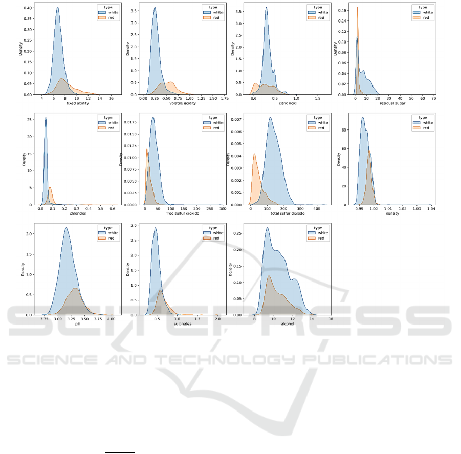
Figure 2: KDE Plots of 11 Features (Picture credit: Original) .

3.1.2 Correlation (Heatmap)

Correlation coefficient is a statistical indicator used to

measure the strength of linear relationship between

variables. The following equation can be used to

calculate the correlation coefficient between two

random variables X and Y.

𝑟

,





∗



(1)

wherein 𝐶𝑜𝑣



𝑋, 𝑌



represents the covariance of X

and Y, 𝜎



and 𝜎



represent standard deviation of X

and Y respectively. Using heatmap to visually

represents the correlations between different

variables in the dataset. The strength of the

correlation is indicated by the intensity of the colour.

The following four machine learning models were

applied on the datasets, and we tried to figure out

which model performs the best with proper

parameters.

Random Forest is composed of numerous

independent decision trees built with random subset

of data and features. It forms the final prediction by

combining the prediction results of all decision trees

through majority voting for classification or weighted

average for regression. By integrating multiple

models, it can effectively mitigate overfitting

problems, improve the prediction accuracy and

generalization ability of the model (Jain et al., 2023

& Zhao and Jiang, 2016).

SVM: finding a hyperplane that maximizes the

margin between classes is the fundamental principle

of SVM, which helps to achieve good classification

performance (Jain et al., 2022).

 Assuming the equation of the hyperplane is:



∗xb0, wherein w is normal vector, b

is the intercept and x is the input features.

 Support vectors are the data points closest to the

hyperplane, which determine the position of the

hyperplane. Support vectors meet the following

conditions: y







∗x



b



1. y



is the class

label of data point x



. The value of y



is either 1

or -1.

(Artificial) Neural Network (NN)/Multilayer

Perceptron (MLP) is a computing architecture based

on human brain functional models, consisting of a set

of processing units called “nodes”. These nodes

transmit data to each other, just like neurons in the

IAMPA 2024 - International Conference on Innovations in Applied Mathematics, Physics and Astronomy

brain transmit electrical pulses to each other. Nodes

are distributed on at least three layers, namely input

layer, hidden layers, and output layer.

XGBoost makes enhancements based on Gradient

Boosting Decision Tree (GBDT), an ensemble

learning algorithm, which optimizes base learners

iteratively and ultimately forms the final strong

learner. Unlike traditional GBDT, XGBoost adds a

regularization term to avoid overfitting.

4 RESULT

4.1 Experiments & Performance

Measurement Setup

The dataset used in this paper is from Kaggle.

There’re 6497 samples in the dataset, 1599 samples

for red wine and 4898 samples for white wine. From

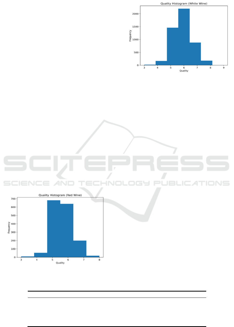
the following figure 3 and figure 4, we found the

distribution of the target (quality scores) is

unbalanced. Unbalanced class distributions present a

barrier to many machine learning algorithms. So, we

used oversampling technique, which adds more

samples from the minority class, to mitigate the

impact of imbalanced classes. Oversampling is

crucial for improving model performance, reducing

overfitting tendencies and enhancing model

generalization ability and robustness. This paper will

discuss the models on red and white wine datasets

separately.

Figure 3: Histogram of Quality Scores (Red Wine) (Picture

credit: Original).

Figure 4: Histogram of Quality Scores (White Wine)

(Picture credit: Original)

In order to measure the performance of machine

learning algorithms, the following performance

measurements are used in the article.

 Accuracy: the percentage of correctly classified

samples by the classifier relative to the total

samples.

 Precision: the percentage of correctly classified

samples by the classifier relative to the positive

samples determined by the classifier.

 Recall: the percentage of correctly classified

samples by the classifier to all positive samples.

 F1 score: the weighted harmonic average of

Precision and Recall.

 AUC: Area Under Receiver Operating

Characteristic (ROC) curve.

The larger the above measurements, the better the

predictive ability of the model.

The (optimal) (hyper)parameters in each machine

learning model for red wine and white wine data are

set through parameter tuning with grid search and

cross validation.

4.2 Experiments Evaluation Analysis

The table 1 and table 2 summarized different

performance measurements for four machine learning

models on red and white wine dataset separately.

Table 1: Performance Measurements Summary for different Machine Learning Models (Red Wine Data).

Machine Learnin

Models Accurac

Precision Recall F1-score AUC

SVM 81.17% 80.76% 82.19% 81.16% 96.27%

RF 90.71% 90.93% 91.38% 91.02% 98.94%

XGBoost 89.49% 89.71% 90.23% 89.70% 98.66%

MLP 79.34% 78.45% 80.49% 79.15% 95.58%

Machine Learning-Based Wine Quality Predictive Modelling

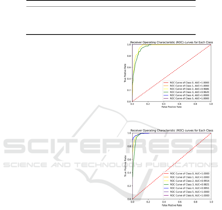
Table 2: Performance Measurements Summary for different Machine Learning Models (White Wine Data).

Machine Learnin

Models Accurac

Precision Recall F1-score AUC

SVM 77.65% 76.76% 77.62% 76.93% 95.68%

RF 93.79% 93.63% 93.71% 93.60% 99.54%

XGBoost 93.01% 92.76% 92.93% 92.76% 99.32%

MLP 80.31% 79.16% 80.14% 79.47% 95.94%

Since different performance measurements have

similar comparison result among four machine

learning models, we will talk about the experiments

based on one measurement, accuracy.

Based on result summarized in Table 1 and Table

2, we find that Random Forest model performs the

best among four machine learning models both on red

wine dataset and white wine dataset. The

performance of XGBoost model is slightly worse than

Random Forest, but better than SVM and MLP. Since

RF and XGBoost belong to ensemble learning, which

typically achieves superior performance than a single

learner. While for SVM and MLP, there’re many

parameters that need to be adjusted, such as selection

of kernel functions and regularization parameters,

learning rate and the number of neurons in the hidden

layers. The selection of these parameters has a

significant impact on the final results and requires

repeated experiments and adjustment. If the

parameters are not selected properly, it may lead to

poor model performance. Moreover, SVM is more

suitable for binary classification problems. For multi-

classes classification problems, multiple binary

classification processes are required.

ROC curve is the curve that present the

relationship between TPR (True Positive Rate) and

FPR (False Positive Rate) under different thresholds.

Since the ROC curve is suitable for binary

classification problem, while our task is a multi-

classification problem. So, we plotted the ROC curve

with some adjustments.

 Plot the ROC curves for different classes

with the optimal machine learning model

Figure 5: ROC curves for different classes with Random

Forest model (Red Wine Data) (Picture credit: Original)

Figure 6: ROC curves for different classes with Random

Forest model(White Wine Data)(Picture credit: Original).

Based on the above figure 5 and figure 6, Random

Forest, which is the optimal model with both red and

white wine dataset, has better predictive ability in

minority classes than majority classes, even though

predictive ability on majority classes is already quite

good. Since we focus more on the minority and

oversampling on minority classes also contributes to

the model, the model is suitable for wine quality

prediction.

IAMPA 2024 - International Conference on Innovations in Applied Mathematics, Physics and Astronomy

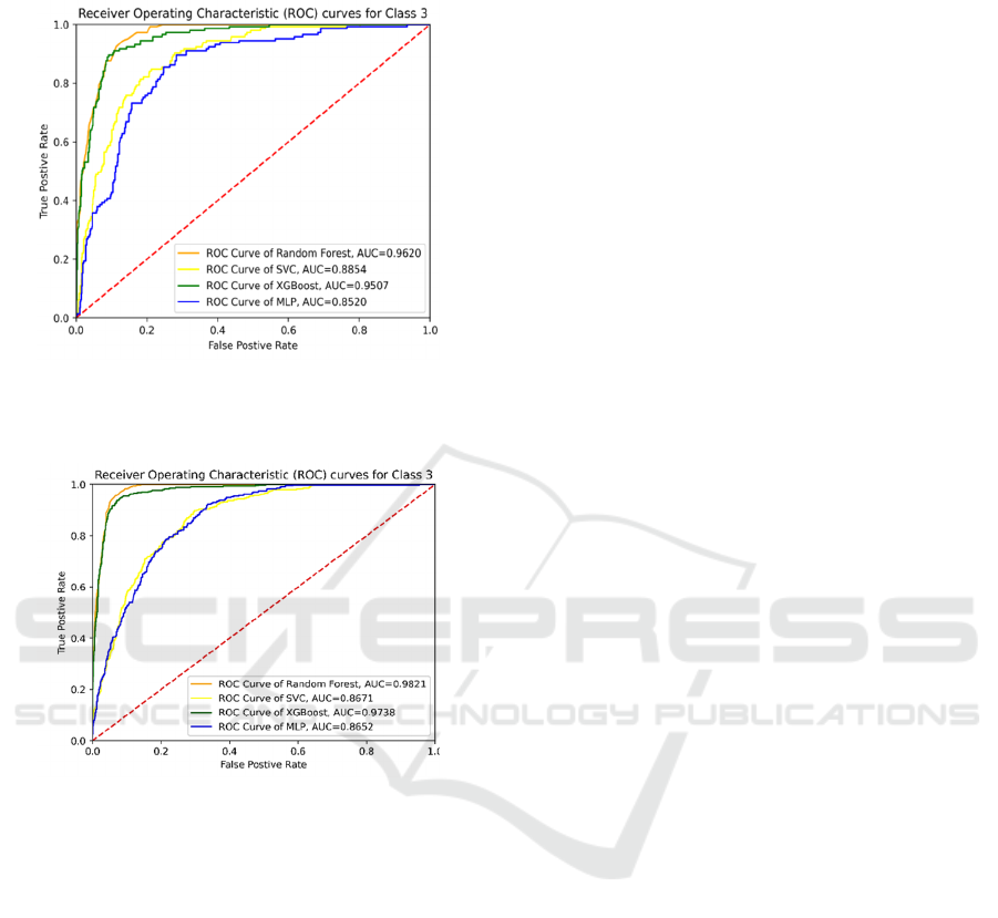
 Plot the ROC curves for a specific class with

four machine learning models

Figure 7: ROC curves for a Specific Class with 4 Machine

Learning Models (Red Wine Data) (Picture credit:

Original).

Figure 8: ROC curves for a Specific Class with 4 Machine

Learning Models (Picture credit: Original).

The larger the area under ROC curve, the better the

performance of the classifier. Based on the above

figure 7 and figure 8, we found that for a specific

class/category both in red and white wine dataset, RF

performs the best. XGBoost performs slightly worse

than RF, but better than SVC and MLP, which also

conforms to the comparison results summarized in

Table 1 and 2.

5 CONCLUSION

In this study, we conducted an in-depth analysis using

samples from both red and white wine datasets,

focusing on eleven physicochemical properties to

construct four machine learning models. The

classifiers' performance was assessed using various

metrics such as accuracy, precision, recall, F1 scores,

and ROC curves to provide a comprehensive

evaluation of the models. Through oversampling and

parameter tuning, we identified Random Forest as the

optimal machine learning model for both red and

white wine datasets, achieving an accuracy score of

90.71% and 93.01% respectively.

Furthermore, our results indicated that XGBoost

outperformed SVM and MLP in the remaining three

models, underscoring the importance of

oversampling in enhancing models' performance.

However, there are still opportunities for

improvement in this research. For instance, further

exploration of feature engineering techniques and

consideration of additional parameters during the

parameter adjustment process could lead to more

robust and accurate models. This highlights the

potential for future research to optimize and refine the

predictive capabilities of machine learning models in

the context of wine quality assessment.

REFERENCES

Zhang, Z., et al. Sensory Quality Evaluation and

Physicochemical Factor Analysis of Wine. Modern

Food 2022, (07), 202-206.

Cheng, Z., et al. A Grading Evaluation Model for Wine

Quality. Science & Technology Industry Parks 2018,

(03), 58.

Yao Y., et al. Research on Wine Evaluation Based on

LASSO Regression. Journal of Yunnan Agricultural

University (Natural Science), 2016,31(02):294-302.

Cortez P., Cerdeira A., Almeida F., et al. Modeling wine

preferences by data mining from physicochemical

properties. Decision Support Systems,2009,47(4):547-

553.

Xia, M., et al. Wine Quality Prediction Based on Support

Vector Machine. Manufacturing Automation 2020,

(05), 57-60.

Zhao, F., & Jiang, S. Application of GA-BP based on

Optimization in Wine Quality Prediction. Journal of

Harbin University of Commerce 2021, (03), 307-313.

Sun W. BP Model After Genetic Algorithm Dimensionality

Reduction Optimization and Wine Quality Prediction.

Journal of Shaoyang College (Natural Science Edition),

2017,14(01):23-29.

Jain, K., et al. Machine Learning-based Predictive

Modelling for the Enhancement of Wine Quality.

Scientific Reports,2023.

Zhang, Z., et al. Machine Learning Approaches for Wine

Quality Prediction. Journal of Food Engineering 2019,

(08), 123-129.

Cheng, Z., et al. Comparative Study of Wine Quality

Evaluation Methods. Food Science and Technology

2017, (06), 45-50.

Machine Learning-Based Wine Quality Predictive Modelling

Xia, M., et al. Feature Selection Techniques for Wine

Quality Prediction. Computers in Industry 2018, (04),

89-94.

Zhao, F., & Jiang, S. Hybrid Model for Wine Quality

Assessment. International Journal of Food Science

2016, (10), 200-205.

Jain, K., et al. Deep Learning Models for Wine Quality

Enhancement. Neural Processing Letters 2022, (02),

75-80.

IAMPA 2024 - International Conference on Innovations in Applied Mathematics, Physics and Astronomy