Prediction of the West Texas Intermediate Crude Oil Price Using
ARIMA Model and ARIMA-GARCH Model
Minzhao Li
School of Statistics and Management, Shanghai University of Finance and Economics, Shanghai, 200082, China
Keywords: Prediction, WTI Crude, ARIMA Model, GARCH Model.
Abstract: Crude oil stands as a pivotal energy source and raw material indispensable for modern life and various
production activities. The fluctuations in its price are intricately linked to the seamless functioning of the
macroeconomy, the healthy development of the capital market, and the choices of individual investors.
However, under the influence of various external factors, international crude oil price changes are
characterized by complexity and are very difficult to predict. This study delves into the monthly fluctuations
of West Texas Intermediate (WTI) crude oil prices, employing the ARIMA and GARCH models to shed light
on its future trajectory. Methodically, it subjects the data to normality tests, stationarity tests, and white noise
tests, while leveraging the AIC information criterion and minimum MSE criterion to fine-tune the model.
Through rigorous analysis, the study establishes both ARIMA (1,1,0) and ARIMA(1,1,0)-GARCH (1,1)
models and both models forecast a modest uptick in oil prices over the next three months, spanning May,
June, and July of 2024. This article adds GARCH model and comparing with the traditional ARIMA model,
ARIMA-GARCH model takes conditional heteroskedasticity into account and can be more accurate and
comprehensive in prediction, which can provide certain reference and suggestion for various investors.
1 INTRODUCTION
In recent years, driven by economic globalization,
crude oil has asserted increasing dominance within
the commodity market. Given its unique
characteristics, the fluctuations and trajectories of
international oil prices have garnered significant
attention. These fluctuations reverberate across
various sectors, impacting government policies,
economic activities, portfolio management, risk
mitigation, and more. Bastianin et al. asserted that
economic policies and financial regulatory measures
aimed at alleviating the adverse consequences of
unforeseen oil price fluctuations should prioritize
addressing the underlying causes of such shocks
(Bastianin et al. 2016). Additionally, the impact of
WTI crude oil price on Shanghai crude oil futures
prices is asymmetric in both intensity and direction in
the short and long term, with a positive effect in the
short term and a negative effect in the long term
(Ding, 2024).
Especially since the advent of the 21st century,
with the advancement of global trade liberalization
and the deepening of world economic globalization,
the crude oil market has witnessed heightened
frequency of fluctuations, resulting in significant
volatility in crude oil prices. This market exhibits
perpetual volatility, marked by conspicuous non-
linearity and pronounced price swings. As a
commodity, crude oil's financial characteristics have
gained prominence, attributed to its pricing
mechanism and the proliferation of derivatives in
financial markets. The dual nature of crude oil renders
its price susceptible not only to market fundamentals
such as supply and demand dynamics and inventory
changes but also to various other influencing factors,
including fluctuations in the U.S. dollar, geopolitical
tensions, economic policies, speculative forces, and
more. However, there are many factors that affect
crude oil, and the inherent relationship between the
various influencing factors is complex. How to
determine the main influencing factors and long-term
influencing factors is a difficult problem.
Sari et al. found that long-term trends in oil prices
are significantly impacted by global risk perceptions
(Sari et al., 2011). Additionally, Le et al. posited that
increases in Covid-19 cases, uncertainties
surrounding U.S. economic policies, and anticipated
stock market volatility collectively contributed to the
decline in WTI crude oil prices in April 2020. Despite
110
Li, M.
Prediction of the West Texas Intermediate Crude Oil Price Using ARIMA Model and ARIMA-GARCH Model.
DOI: 10.5220/0012999200004601
Paper published under CC license (CC BY-NC-ND 4.0)
In Proceedings of the 1st International Conference on Innovations in Applied Mathematics, Physics and Astronomy (IAMPA 2024), pages 110-118
ISBN: 978-989-758-722-1
Proceedings Copyright © 2024 by SCITEPRESS – Science and Technology Publications, Lda.

these challenges, losses in global stock markets
appeared to have been notably mitigated (Le et al.,
2021). Wang et al. argued that in extreme scenarios,
there exists a robust causal relationship between
investor sentiment and the crude oil futures market
(Wang et al., 2021).
Therefore, how to accurately predict WTI crude oil
prices has become a top priority, and many complex
and innovative models have been built to predict WTI
crude oil prices. Traditional econometric models play
a crucial role across diverse economic domains,
including the prediction of WTI crude oil prices.
Herrera employed RiskMetrics and GARCH models
for short-term forecasts, Exponential GARCH
(EGARCH) for medium-term horizons, and Markov-
switching GARCH (MS-GARCH) for long-term
predictions (Wang and Liu, 2016 & Herrera, Hu and
Pastor, 2018). Indeed, machine learning methods and
hybrid models have gained significant traction in the
realm of crude oil price prediction. A multitude of
scholars have conducted extensive research in this
area. Wu et al. leveraged a Convolutional Neural
Network (CNN) model to extract text features from
news media texts and Google Trends data, assessing
their efficacy in explaining crude oil price predictions
(Wu et al., 2021). Li et al. investigated the enduring
impacts of global crude oil production and economic
activities on crude oil prices. They devised a hybrid
model incorporating Genetic Algorithm Optimized
Support Vector Machine (GASVM) and Back
Propagation Neural Network (BPNN) to analyze
monthly oil price data for predictive purposes (Li,
Zhu and Wu, 2019). Wang fused a multi-layer
perceptron with a neural network to develop an
Elman Recurrent Neural Network (ERNN) model for
empirical crude oil price forecasting (Wang and
Wang, 2016).
Overall, these studies highlight the need for
accurate prediction of the global price of WTI crude.
The econometric model can predict short-term crude
oil prices more accurately, but the nonlinear, complex
and non-stationary characteristics of crude oil prices
make the model have certain flaws. The machine
learning model uses linear and nonlinear models to
enrich the experimental process and set up various
scenarios to improve the applicability of the model.
Then, more complex deep learning models and
numerous neural network algorithms were added to
forecasts, which can extract effective information and
focus on trends and changes in time series. This paper
will primarily concentrate on utilizing the ARIMA
and GARCH models for crude oil price prediction.
The aim is to offer a valuable reference for crude oil
futures investors, aiding them in making informed
decisions and conducting risk mitigation transactions.
By leveraging these models, investors can potentially
reduce their losses to a considerable extent.
2 METHODOLOGY
2.1 Data Source
Fred's global WTI crude oil price index is the source
of the data used in this investigation. This dataset
comprises monthly average prices of crude oil in U.S.
dollars. It is meticulously documented, with no
instances of missing values or outliers. For analysis,
the paper has selected price data spanning from
January 2000 to April 2024, amounting to 292
observations. The first 276 observations, covering the
period from January 2000 to December 2022,
constitute the training set, while the remaining 16
observations, spanning from January 2023 to April
2024, are designated as the test set. Ultimately, a
rolling forecast approach is adopted to predict the
WTI crude oil price for May, June, and July 2024.
The internationally recognized crude oil
benchmark prices are WTI and Bren crude oil prices.
This paper selects the price of WTI crude oil, which
occupies the leading position in terms of global
commodity futures trading volume because of its
advantages of transparent quotations and high
liquidity, as well as the status of U.S. super crude oil
buyers and the world influence of the New York
Stock Exchange. At the same time, this paper selected
prices rather than yields, average prices rather than
closing prices, and monthly data over the past decade
rather than all data.
2.2 Variable Selection
Crude oil prices are obviously volatile and cyclical.
Indeed, the prices of crude oil can experience
substantial fluctuations, with the potential for
significant rises or falls within relatively brief time
frames, and they can experience rising and falling
cycles over a span of several years or even ten years.
Changes in oil prices are often affected by
geopolitics, technological progress, and the
macroeconomic environment, as illustrated in Figure
1:
Prediction of the West Texas Intermediate Crude Oil Price Using ARIMA Model and ARIMA-GARCH Model
111

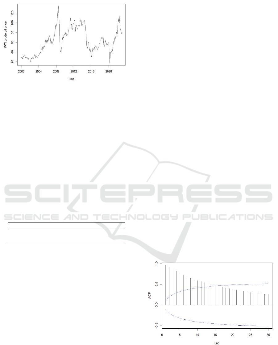
Figure 1: Global WTI crude price.
From Figure 1, it can be concluded that WTI oil
prices remained slightly unchanged from 2000 to
2004, then gradually increased, reaching their peak in
the summer of 2008 due to geopolitical tensions, and
then rapidly collapsing due to the impact of the 2008
financial crisis. , then prices rose slowly from 2009 to
2014, then dropped rapidly due to excess production,
then gradually climbed higher from 2016 to 2020, and
then plummeted rapidly in 2020 because of the
COVID-19 pandemic's effects. It has risen rapidly in
the past three years and declined rapidly in the past
year. This article uses a univariate time series. The
selection of variables is shown in Table 1. Month is
used as the time series and price is used as the
variable.
Table 1: List of Variables.
Variable Type Meaning
Month Date Month
WTI Double WTI crude oil
p
rice
(
dollar
)
2.3 Model Selection
This article uses Autoregressive Integrated Moving
Average (ARIMA) and Generalized Autoregressive
Conditional Heteroskedasticity (GARCH) models to
process time series data of crude oil prices. ARIMA
consists of autoregression (AR), difference (I) and
moving average (MA). The AR part contains the
impact of observations from past periods on current
values. Part I transforms non-stationary time series
into stationary by removing trends and seasonal
characteristics through differencing. The MA part
takes into account the impact of past forecast errors
on the current value. The GARCH model is also
called the generalized ARCH model. It not only takes
into account the volatility aggregation phenomenon
caused by the heteroscedasticity of the sequence like
ARCH, but also takes into account several lag terms
of the variance to capture more heteroskedasticity
information.
3 RESULTS AND DISCUSSION
3.1 Data Processing
The data used to build the model need to be
stationary. First, it is necessary to determine whether
the original sequence data is stationary. By observing
the time series diagram in Figure 1, the ACF diagram
(Figure 2), and performing the ADF unit root test, we
can see that the model is not stationary. For this
purpose, it is necessary to stabilize by difference
processing or logarithmic transformation processing.
First, first-order difference processing is used. By
analysing the timing diagram (Figure 3), ACF
diagram, and PACF diagram (Figure 4) after first-
order difference, we can conclude that the series has
already been stationary and there is no need to
perform second-order difference or logarithmic
transformation. Besides, according to Table 2, the
ADF test shows that when the lag order is chosen to
be 1, the sequence is stationary in all three cases:
including time trends and intercept terms, only
intercept terms, and no definite trend (in the first case
the model has already been stationary and for
accuracy, the other two cases are also tested).
Besides, the lag order 1 is determined step by step
starting from 10 and the reason why the AIC criterion
is not adopted is to make the test more accurate,
because the AIC criterion cannot guarantee that serial
correlation will be eliminated.
Figure 2: The ACF plot of original sequence.
IAMPA 2024 - International Conference on Innovations in Applied Mathematics, Physics and Astronomy
112

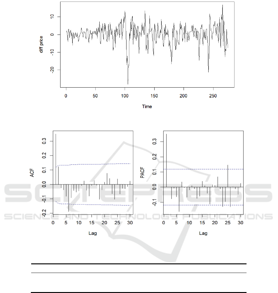
Figure 3: First-order differential timing diagram.
Figure 4: First-order differential ACF plot and PACF plot.
Table 2: The ADF test.
Type Dickey-Fuller Lag order p-value
Intercept + time tren
d
-9.285 1 0.0708
Interce
p
t onl
y
-9.298 1 0.6143
No intercept and tren
d
-9.309 1 0.3368
3.2 Model Evaluation
The selection of p and q parameters can be
determined through the Autocorrelative Function
(ACF) plot and Partial Autocorrelative Function
(PACF) plot (Figure 4). The ACF plot is employed to
ascertain the coefficient (q) of the MA model, while
the PACF plot is utilized to determine the coefficient
(p) of the AR model. By observing the above figure,
it can be seen that both figures exceed the critical
value when lag equals 1 and 6. The models can be
initially identified as ARIMA (0,1,1), ARIMA
(0,1,6), ARIMA (1,1,0), ARIMA (6,1,0). The Akaike
Information Criterion (AIC) is an assessment
criterion that utilizes the notion of information
entropy. It acts as a benchmark for evaluating a
statistical model's complexity and the effectiveness of
model fitting. The degree of model fitting is better the
smaller the AIC. Firstly, fit the above four models
respectively, select the two models with smaller AIC,
ARIMA (1,1,0) and ARIMA (6,1,0) for further
analysis, and then conduct overfitting analysis. For
Prediction of the West Texas Intermediate Crude Oil Price Using ARIMA Model and ARIMA-GARCH Model
113

the two preliminary models, appropriately increase
the order of MA, q, from 0 to 1, and fit the two new
models. It is found that the AIC becomes larger, and
the model is considered to be insufficiently fitted, so
discard them. The AIC of each model are as shown in
Table 3.
Table 3: Model determination.
ARIMA Model AIC
(0,1,1) 1721.40
(
0,1,6
)
1717.89
(1,1,0) 1716.31
(
6,1,0
)
1716.48
Additional model
(
6,1,1
)
1718.21
(1,1,1) 1718.31
3.3 Residual Analysis
In order to test the quality of the fitted model, residual
analysis is needed. If the model identification is
correct, the characteristics of the residuals are similar
to those of the white noise sequence, and similar to
independent and identically distributed normal
random variables. First, check whether the residual
sequence contains a trend that is not explained by the
fitted model by observing the time series plot, then
check whether normality is satisfied through the QQ
plot and normal distribution test, and finally check
whether the normality is satisfied through the ACF
plot, PACF plot and Ljung-Box Test to check for
autocorrelation.
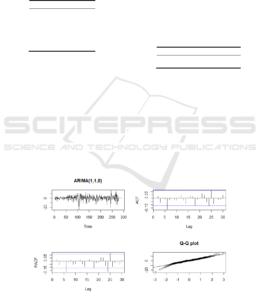
It can be seen from Figure 5 that the residual timing
diagram fluctuates up and down at 0. In both the ACF
plot and the PACF plot, the values exceed the critical
value when the lag order is 6, and also slightly exceed
it when the lag order is larger (negligible). It can be
seen from the QQ plot that there are a few abnormal
points that do not adhere to a normal distribution. The
p-value of the Shapiro-Wilk (SW) test in Table 4 is
small (0.000013) so residuals do not adhere to a
normal distribution. The Ljung-Box (LB) test values
in Table 5 are basically greater than 0.2 except one,
so it can be considered that there is no
autocorrelation.
Table 4: Shapiro-Wilk test.
Model W p-value
ARIMA
(
1,1,0
)
0.9711 0.000013
ARIMA(6,1,0) 0.9748 0.000051
Figure 6 makes it clear that the residual timing
diagram fluctuates up and down at 0. In both the ACF
plot and the PACF plot, the values slightly exceed the
critical value when the lag order is larger than 15
(negligible). It can be seen from the QQ plot that there
are a few abnormal points that do not obey the normal
distribution. Because of the modest p-value
(0.000051) of the SW test in Table 4, the residuals do
not follow a normal distribution. Table 5's LB test
results are unquestionably higher than 0.2, so it can
be definitely considered that there is no
autocorrelation.
Figure 5: ARIMA (1,1,0) residuals plot, ACF plot, PACF plot, QQ plot.
IAMPA 2024 - International Conference on Innovations in Applied Mathematics, Physics and Astronomy
114

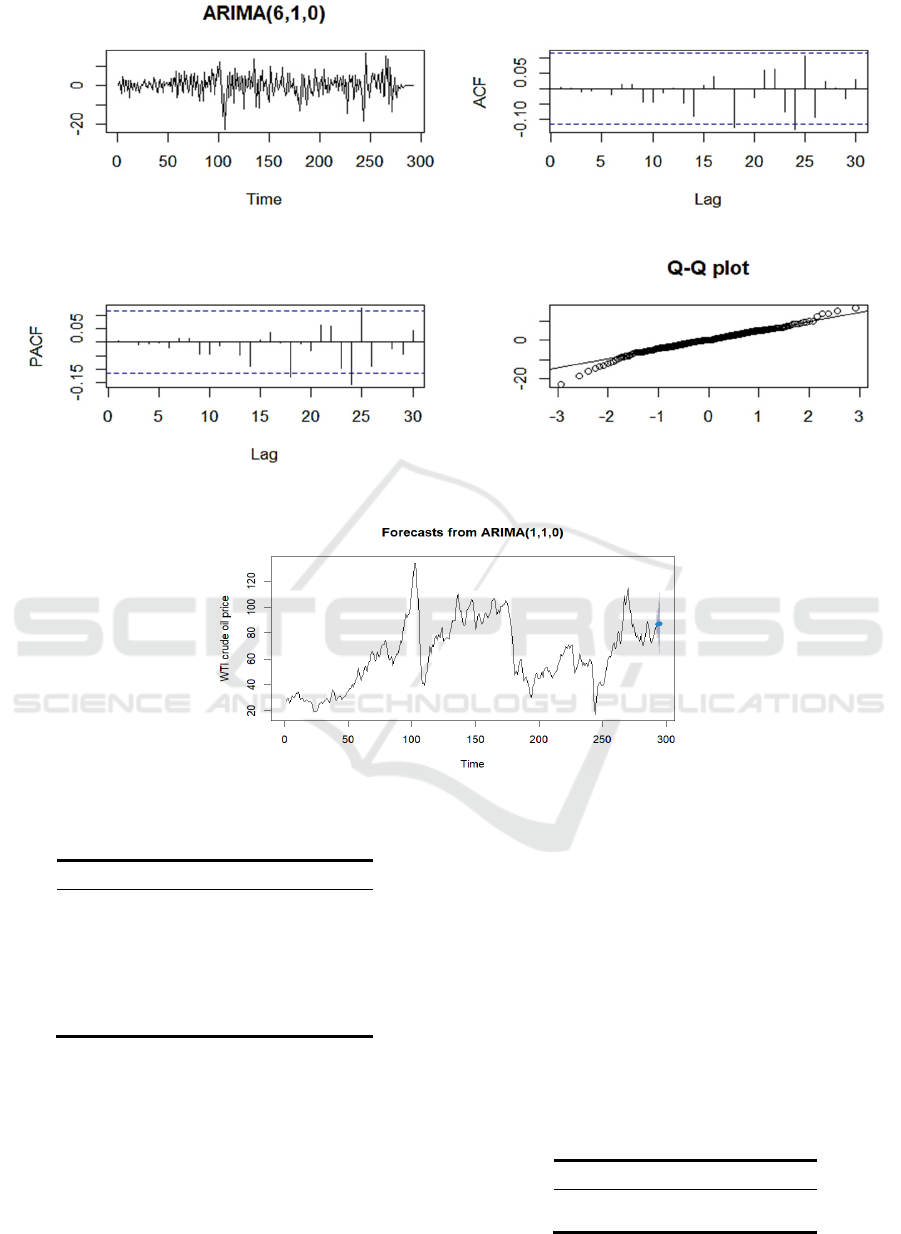
Figure 6: ARIMA (6,1,0) residuals plot, ACF plot, PACF plot, QQ plot.
Figure 7: Forecasts from ARIMA (1,1,0).
Table 5: Ljung-Box test.
Model Q* df p-value
ARIMA(1,1,0) 10.160 6 0.071
11.737 12 0.384
18.955 18 0.331
27.399 24 0.239
ARIMA(6,1,0) 1.4920 12 0.960
10.019 18 0.614
19.929 24 0.337
3.4 Forecasting
The next process is to verify the model and make
predictions. This article uses rolling forecast and
sliding window width instead of multi-step forward
forecast. The purpose is to incorporate the latest data
points for more accurate forecasts. Because the
ARIMA model is only suitable for short-term
forecasts, the effect of multi-step forward forecast is
often not good. good. First, establish the above two
models for the training set, only perform one-step
forward prediction, then incorporate a new test set
data point (without deleting old data points), fit the
model again, continue prediction, and repeat the
above process 16 times. Then use mean square error
(MSE) and mean absolute error (MAE) to verify the
model fitting effect. A smaller value for both
coefficients indicates better performance of the model
on the test set. The MSE and MAE of ARIMA (1,1,0)
and ARIMA (6,1,0) are shown in Table 6:
Table 6: Model validation.
Model MSE MAE
ARIMA(1,1,0) 27.615 4.676
ARIMA
(
6,1,0
)
31.894 5.015
Prediction of the West Texas Intermediate Crude Oil Price Using ARIMA Model and ARIMA-GARCH Model
115

It can be seen that the MSE and MAE of ARIMA
(1,1,0) are smaller and the model fitting effect is
better, so it is used as the final model to predict WTI
crude price. The last step is to predict the latest
unknown data points. The crude oil price forecast for
the latest three months is shown in Figure 7 and Table
7:
Table 7: Forecasts from ARIMA (1,1,0).
Time Point
forecast
L 80 H 80 L 95 H 95
2024
/
05 86.705 79.754 93.656 76.075 97.336
2024/06 87.173 75.525 98.821 69.360 104.987
2024/07 87.334 71.871 102.798 63.685 110.984
The blue plots show the forecasting value and the
grey area shows the model's prediction limit at
confidence levels of 80 and 95. From the findings
above, it is evident that the predicted oil price
experienced a slight increase in the next three months.
3.5 GARCH Model
It should be noted that a prerequisite of the ARIMA
model is that the data is conditionally homoscedastic.
However, for many financial time series data, such as
the WTI crude oil price analysed in this article, their
conditional variance is affected by the present and the
past, and has Conditional heteroskedasticity. This
kind of data has the characteristic of continuous peaks
and troughs: large fluctuations are often succeeded by
subsequent large fluctuations, while small
fluctuations tend to be followed by additional small
fluctuations. Therefore, it is necessary to use the
GARCH model to model the variance of the data.
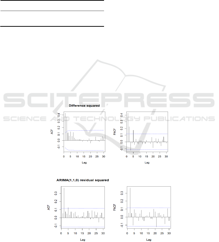
To determine whether the model exhibits
heteroscedasticity, it is essential to observe the ACF
and PACF plots of the square of the sequence after
the difference and the square of the residual after
fitting the model. If there is a significant correlation,
it indicates the existence of conditional
heteroskedasticity. As shown in Figure 8 and Figure
9, the squared plot of the differential sequence
exceeds the critical value many times when the lag
order is 1 to 5. The residual squared sequence also
significantly exceeds the critical value when the lag
order is 2 in the two figures. It can be considered that
there is a conditional difference. variance. At the
same time, McLeod-Li test, one of the white noise
tests, is performed on the square sequence. According
to Figure 10, the point values are all lower than the p
value of 0.05, which is also considered to have
conditional heteroskedasticity.
Figure 8. The ACF plot and PACF plot of difference squared.
Figure 9: The ACF plot and PACF plot of ARIMA (1,1,0) residual squared.
IAMPA 2024 - International Conference on Innovations in Applied Mathematics, Physics and Astronomy
116

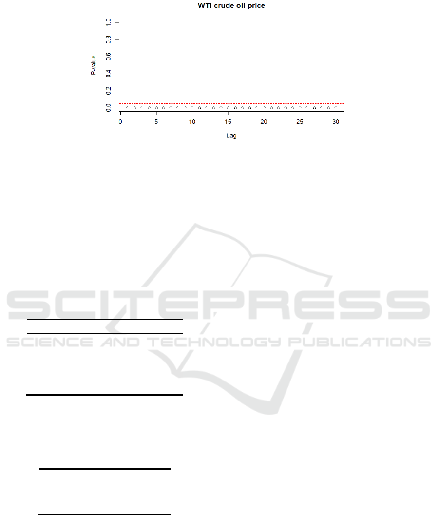
Figure 10: The ACF plot and PACF plot of ARIMA (1,1,0) residual squared.
Considering conditional heteroskedasticity, an
ARIMA-GARCH model is established to fit the data,
and the ARIMA (1,1,0) determined previously and
the GARCH (1, 1) most commonly used for financial
time series data are combined to fit the WTI crude oil
price data. Then, carry out residual analysis and
conduct Ljung-Box test on residual and residual
square respectively to test the fitting effect of ARIMA
model and GARCH model. As can be seen from
Table 8, the p values are large, both are greater than
0.1, and it can be considered that the fit is good.
Table 8: Ljung-Box test for ARIMA-GARCH model.
Object Q* df p-value
residual 2.305 1 0.129
2.307 2 0.128
2.846 5 0.471
Residual s
q
uare
d
0.074 1 0.785
2.475 5 0.511
4.093 9 0.573
Results of the predictions are displayed in Table
9. It is evident that throughout the next three months,
oil prices will continue to rise marginally.
Table 9: Forecasts from ARIMA (1,1,0)-GARCH (1,1).
Time Point forecast Sigma
2024
/
05 86.140 4.989
2024/06 86.299 5.067
2024/07 86.331 5.144
3.6 Critical Thinking
Although this article is very detailed and
comprehensive in modeling, and combines ARIMA
and GARCH, two very commonly used time series
models, to fit the data, it can be said that the
predictions under this large framework will be very
accurate. But in fact, no one can know which model
the data obeys, especially for financial time series
data, which is characterized by very high volatility
and uncertainty, and is extremely susceptible to
external interference. This article does not consider
derivative models of GARCH, such as Threshold
GARCH (TGARCH) or Asymmetric Power GARCH
(APARCH), etc. It does not take into account the
asymmetric effect and Taylor effect. At the same
time, in terms of machine learning, algorithms such
as CNN and SVM are not integrated into oil price
predictions, and in terms of external factors, there is
no way to take into account the interference of oil
price factors, such as oil supply and demand and
geopolitical risks.
4 CONCLUSION
This article forecasts monthly WTI crude oil prices
using the ARIMA and ARIMA-GARCH models, and
conducts tests such as stationarity test, normality test,
white noise test, and model fitting goodness. The
model is finally determined to be ARIMA (1,1,0) and
ARIMA(1,1,0)-GARCH(1,1) respectively predict
that oil prices will rise slightly and even slightly in the
next three months, that is, in May, June, and July
2024.
However, a variety of factors will affect the price
of crude oil amid the current global economic
downturn. Oil prices will become more difficult to
anticipate due to the production strategies of countries
that produce crude oil, geopolitical events, the
development of new energy technologies, and the
activities of futures markets and commodity
exchange-traded funds, such as exchange traded fund
(ETF) in the financial market. It should be noted that
the research in this article does not take into account
realistic and complex scenarios. For macro managers
Prediction of the West Texas Intermediate Crude Oil Price Using ARIMA Model and ARIMA-GARCH Model
117

who hope that the crude oil futures market will
operate effectively and achieve stable futures prices,
and speculators who hope to have the opportunity to
achieve excess profits, the model selected in this
article is relatively simple. It does not constitute
investment advice and can only be used as a reference
to a certain extent.
REFERENCES
Bastianin A, Conti F and Manera M 2016 The impacts of
oil price shocks on stock market volatility: Evidence
from the G7 countries. Energy Policy, 98 160-169.
Ding X 2024 Research on the asymmetric impact of
international crude oil prices on Shanghai crude oil
futures prices. China-Arab Science and Technology
Forum, 43-47.
Sari R, Soytas U and Hacihasanoglu E 2011 Do global risk
perceptions influence world oil prices? Energy
Economics, 33(3) 515-524.
Le T-H, Le A T and Le H-C 2021 The historic oil price
fluctuation during the Covid-19 pandemic: What are the
causes? Research in International Business and
Finance, 58.
Wang L, Ma F, Niu T J and Liang C 2021 The importance
of extreme shock: Examining the effect of investor
sentiment on the crude oil futures market. Energy
Economics, 99.
Wang Y D and Liu L 2016 Crude oil and world stock
markets: Volatility spillovers, dynamic correlations,
and hedging. Empirical Economics, 50(4) 1481-1509.
Herrera A M, Hu L and Pastor D 2018 Forecasting crude
oil price volatility. International Journal of Forecasting,
34(4) 622-635.
Wu B, Wang L, Lv S, et al. 2021 Effective crude oil price
forecasting using new text-based and big-data driven
model. Measurement, 168.
Li J, Zhu S and Wu Q 2019 Monthly crude oil spot price
forecasting using variational mod decomposition.
Energy Economics, 83 240-253.
Wang J and Wang J 2016 Forecasting energy market
indices with recurrent neural networks: Case study of
crude oil price fluctuations. Energy, 102 365-374.
IAMPA 2024 - International Conference on Innovations in Applied Mathematics, Physics and Astronomy
118