Nonlinear Control and State Estimation for the Hand Axes of a
Pneumatic Robot
Seyed Houman Mirafzal
Independent Researcher, Germany
Keywords: Mechatronics, Robotics, Predictive Control, Flatness-Based Methods, Pneumatic Muscle.
Abstract: This paper presents a nonlinear control for the hand axes of a robot with three pneumatic muscles. A vector-
based approach is employed for the modeling. Due to the structure of the system, a flatness-based control
method is chosen and used. A control system is designed in which three types of compensators, including
feedback, feedforward, and observer (estimator) are used to improve the trajectory tracking of the main joint
angles and the muscle force control. The Kalman Filter is used to estimate the disturbance friction torque in
the system. Through a combination of theoretical analysis and experimental validation, the proposed methods
demonstrate significant improvements in control accuracy and system stability. As a result, the control system
tracks the desired trajectories very well, as various trajectories are implemented to test the tracking behavior
of the control system.
1 INTRODUCTION
The integration of automatic control systems has
become pivotal in modern industries, enhancing both
efficiency and precision across a wide range of
applications. While open-loop control systems suffice
for the operation of simpler devices, such as
household appliances, the demand for increasingly
complex feedback control systems has steadily
grown. Feedback control systems, which
continuously monitor and adjust outputs to align with
desired set points, are essential for high-precision
tasks, ranging from industrial automation to delicate
surgical procedures.
Although control using electric actuators is more
common due to its processing flexibility, pneumatic
control, which operates based on the pressure and
force of compressed air, remains crucial in modern
industry (Franklin et al., 2019). Pneumatic actuators
are commonly used in automation and robotics due to
their lightweight and naturally compliant behavior,
which comes from air's compressibility. This
compliance, adjustable through pressure control, is
essential for safe human-machine interactions and
delicate tasks like handling fragile objects. In
contrast, hydraulic and electric systems are more rigid
and require relatively more complex feedback control
to achieve similar flexibility (Daerden et al., 2002). In
addition, because pneumatic muscles can produce
relatively big forces and make these forces last long
without much effort, using them is also advantageous
(Schindele et al., 2013).
Pneumatic robots, characterized by their inherent
compliance and safety, present unique challenges in
control due to their nonlinear behavior and dynamic
uncertainties. These robots are particularly
advantageous in environments where human-robot
interaction is frequent, as their compliant nature
reduces the risk of injury. However, the nonlinear
dynamics of pneumatic actuators necessitate
advanced control strategies to achieve precise and
reliable performance.
This experiment addresses the critical need for
robust nonlinear control and state estimation
techniques for the hand axes of a pneumatic robot, in
which the axes of the three pneumatic muscles are
regarded as the axes of the robot hand. The
experiment aims for optimization of the control
process by merging all the compensators (feedback,
feedforward, and observer) together, while the model
is also considered as similar as possible to the real
physical system.
Figure 1 shows two images of the robot, in which
its main components are introduced, while the
muscles are still not filled with the compressed air. A
comprehensive approach is proposed that includes the
development
of nonlinear controllers designed to
236
Mirafzal, S.
Nonlinear Control and State Estimation for the Hand Axes of a Pneumatic Robot.
DOI: 10.5220/0013006500003822
Paper published under CC license (CC BY-NC-ND 4.0)
In Proceedings of the 21st International Conference on Informatics in Control, Automation and Robotics (ICINCO 2024) - Volume 2, pages 236-247
ISBN: 978-989-758-717-7; ISSN: 2184-2809
Proceedings Copyright © 2024 by SCITEPRESS – Science and Technology Publications, Lda.

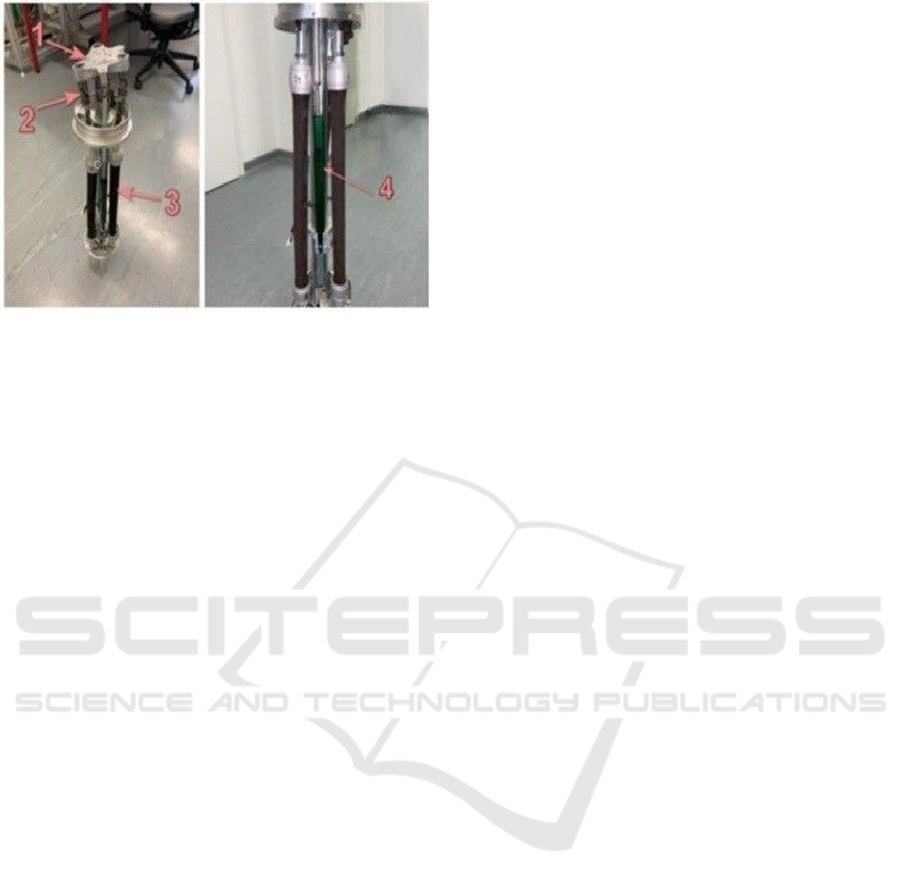
Figure 1: The pneumatic robot. The system consists of four
major parts: the joint top plate (1), the joint level (2), the
three pneumatic muscles (3) and the two measuring
cylinders or potentiometer sensors (4).
enhance trajectory tracking and force control
accuracy.
This paper is structured as follows: First, the
system is modeled using vectors and various
coordinate systems to simplify calculations. While
some components, like the chains and fully realistic
top plate, are approximated, the model closely
represents the real system, resulting in minimal
residual errors. Multiple coordinate systems, tailored
to the shape, degrees of freedom, and movement
directions, make the modeling and logic easier to
understand. Transformation matrices facilitate easy
variable transfers between coordinate systems. Next,
the equations for modeling the pneumatic muscles,
including required coefficients, are derived
experimentally.
New coefficients and muscle
characteristics specific to this system are calculated.
Furthermore, flatness-based controllers are designed
for the desired control response. Initial controllers
manage angles that approximate the rotated top plate
angles. Secondary controllers manage the pneumatic
system, controlling muscle forces based on desired
torques and mean force. Moreover, the desired
trajectories and feasible variable ranges, considering
the real physical system, are explained. Movement,
pressure, and force limitations in the pneumatic
system are detailed, such as restricted rotation angles
of the top plate and pressure limits affecting muscle
forces. As the air mass flow rate 𝑚 is considered the
manipulated variable of the control system, the initial
and the maximum air pressure in the muscles are
considered 1 bar and 8 bars, respectively.
Additionally, data derived from plotting the results in
MATLAB/Simulink indicate that the desired mean
force should not fall below 15 newtons to ensure
logical system responses. Observers are also used to
estimate and compensate for friction as a disturbance.
The Kalman Filter is chosen as an optimal method
among various observer options. Finally, the entire
control system model is evaluated regarding its
responses and results, comparing them to expected
outcomes. As a result, it is shown that the desired
trajectories are being tracked fast with a high
accuracy, due to the precise design of the control
system, including different compensators. The paper
concludes by summarizing the thesis aims and
discussing system applications.
2 MULTI-BODY MODELING
As discussed in the introduction, the kinematic
modeling of the robot is based on vectors and
different coordinate systems, corresponding to the
system's parts and their movement directions. The
bottom plate, located at the base of the pneumatic
muscles, remains stationary, so the initial point (O
1
)
of the primary coordinate system (system 1) is set at
the center of this plate.
The main joint, which allows two perpendicular
angular rotations, is located in the middle of the joint
level. These rotation angles are the main controlling
angles. The center of this joint is the center point (O
2
)
of the next coordinate system (system 2), formed by
rotating system 1 around the x-axis by angle 𝜑
1
. The
final coordinate system is created by rotating system
2 around its y-axis (y
2
-axis) by angle 𝜑
2
. Figure 2
shows the simplified system model, including the
three coordinate systems.
The robot hand axes design benefits from
symmetry, simplifying calculations and modeling.
Additionally, the end joints of the pneumatic muscles
are aligned with the main joint's center, further easing
the modeling process.
2.1 Modeling the Hand Axes and the
Pneumatic Actuators
The primary goal in modeling the robot hand axes is
to determine the relationship between the vectors of
the model's different parts, the rotation angles, and the
changes in the lengths of the two potentiometer
sensors, X
10
and X
11
, as shown in figure 1. Since X
10
and X
11
are the only means of measuring the current
positions or lengths of other components, establishing
this relationship is crucial. The modeling process is
conducted in several steps, as described in the
following sections.
Nonlinear Control and State Estimation for the Hand Axes of a Pneumatic Robot
237

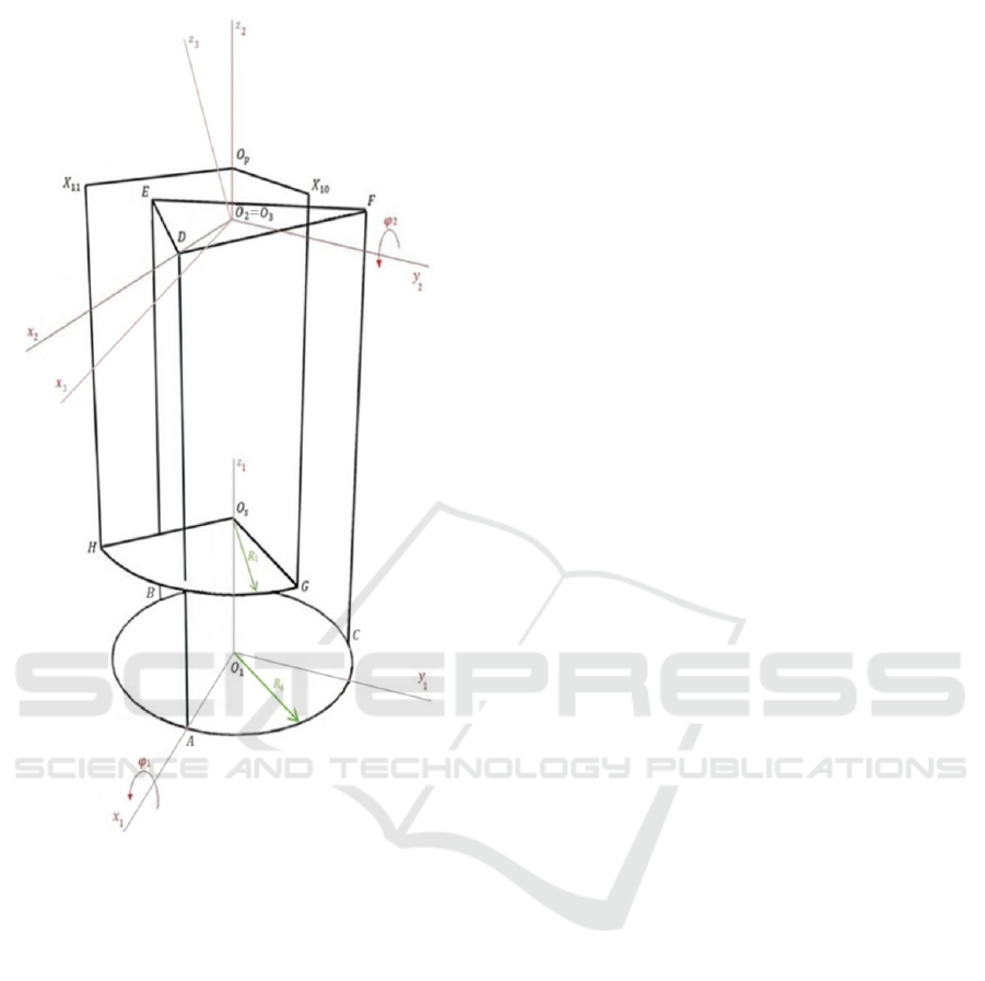
Figure 2: The simplified model, including the bottom
surface of the muscles, top triangular surface and the
sensors’ bottom and top positions.
2.1.1 Selecting Different Coordinate Systems
As mentioned briefly earlier, the modeling involves
three coordinate systems. To explain the system's
behavior better, the second and third coordinate
systems are placed at the main joint just below the top
surface. Key points for calculations include the
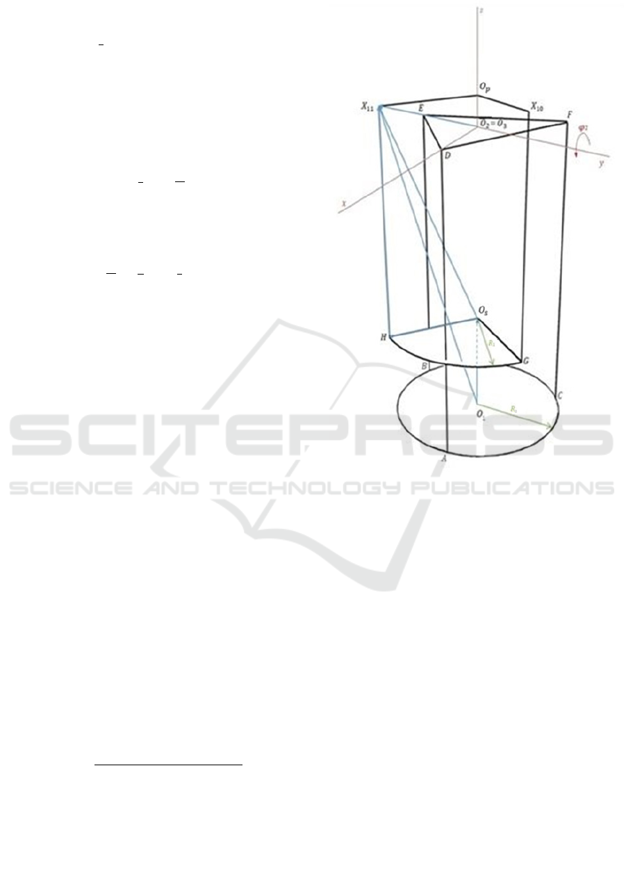
centers of the pneumatic muscle top joints (D, E, and
F), as shown in figure 2.
2.1.2 Vector-Based Modeling
In the modeling approach, muscles and their chains
together are treated as vectors in three-dimensional
space for calculations and coding purposes. As
previously mentioned, the goal is to relate these
vectors to the rotation angles of the main central joint,
O
2
, to the outputs from sensors X
10
and X
11
. For this
purpose, a vector must represent each pneumatic
muscle.
The secondary coordinate system, system 2,
centered at the main joint with origin O
2
, simplifies
calculations for vectors such as
1
𝑟⃗
D 1
, which represent
distances like O
1
to D. These vectors are transformed
into the initial coordinate system using a
straightforward multiplication by a transformation
matrix explained in section 2.1.3.
2.1.3 Derivation of the Transformation
Matrix
In subsection 2.1.2, the concept of representing
vectors in different coordinate systems is introduced.
In order to calculate each vector component in a new
coordinate system, a transformation matrix is
required. The transformation matrix to form a new
coordinate system 3, after two consequent rotations
about x- and y-axes, can be stated as (Woernle,
2016)
13
T =

𝑐𝑜𝑠 𝜑

0𝑠𝑖𝑛 𝜑

𝑠𝑖𝑛 𝜑

𝑠𝑖𝑛 𝜑

𝑐𝑜𝑠 𝜑

− 𝑠𝑖𝑛 𝜑

𝑐𝑜𝑠 𝜑

− 𝑐𝑜𝑠 𝜑

𝑠𝑖𝑛 𝜑

𝑠𝑖𝑛 𝜑

𝑐𝑜𝑠 𝜑

𝑐𝑜𝑠 𝜑

 .
(1)
Similarly, this 2 degrees of freedom (DOF)
system involves rotations around the main center joint
along x- and y-axes. Thus, analogous to the equation
(1), separate transformation matrices are developed:
12
T,
23
T, and
13
T, representing movements between
coordinate systems. Therefore, each vector can be
calculated in the third coordinate system to ease the
calculations, by having its components in the first
coordinate system as follow
1
𝑟⃗ =
13
T .
3
𝑟⃗ .
2.2 Experimental Identification of
Unknown Parameters
Pneumatic systems involve diverse muscle types,
each with specific characteristics like air pressure
requirements for contraction. A key challenge in
pneumatic muscles is hysteresis. This effect in
pneumatic muscles arises from the relative motions
occurring during muscle inflation or deflation, which
increase the system's nonlinearities and complexities
(Vo et al., 2010). Internal friction between the aramid
fibers and the surrounding elastic material also
contributes to hysteresis (Deaconescu et al., 2016).
Despite its potential impact, hysteresis is negligible in
(2)
ICINCO 2024 - 21st International Conference on Informatics in Control, Automation and Robotics
238

this experiment and is omitted in the pneumatic
control model design.
The complete force characteristic F
Mi
can be
stated as (Schindele et al., 2013)
F
Mi
= F
Mi,st
+ F
Mi,hys
,
where F
Mi,st
, and F
Mi,hys
denote the static muscle force
and the hysteresis effect, respectively.
Because the hysteresis effect, F
Mi,hys
, is negligible
in this experiment, therefore, complete force
characteristic F
Mi
is considered approximately equal
to the static muscle force F
Mi,st
. As a result,
F
Mi
≈ F
Mi,st
.
The muscle force depends on internal pressure
𝑝

and contraction length Δ𝑙

approximated by
𝐹
,
(
𝑝

,Δ𝑙

)
=

𝐹


(
𝑝

,Δ𝑙

)
𝑖𝑓 𝐹


0
0 𝑒𝑙𝑠𝑒
,
The amounts of the coefficients 𝑎

and b
n
can be
defined experimentally. The Recursive Least Squares
(RLS) method is a reliable approach for parameter
estimation (Xie et al., 2011), requiring extensive data
collection—about 20,000 states of p
Mi
, 𝛥𝑙
Mi
, and F
Mi
are practically analyzed in the university laboratory.
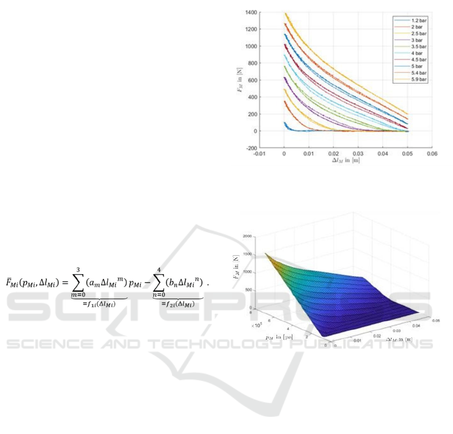
Figure 3 illustrates results for 10 internal muscle
pressures.
By using the RLS method, the quantities for 𝑎

and bn can be calculated.
Consequently, the resulting three-dimensional
figure for the identified force characteristic of the
pneumatic muscle can be plotted as figure 4.
3 DESIGN OF THE NONLINEAR
MIMO AND INVERSE SYSTEM
MODEL
The flatness-based control approach is chosen, due to
the suitable trajectory tracking structure and inclusion
of the feedforward compensator, as it is discussed in
more detail in section 3.
Figure 3: The resulting curves, including the relationship
between the created muscle force and the contraction length
for 10 different pressures.
Figure 4: The force characteristic of the pneumatic muscle.
In order to design a complete flatness-based
feedback cascade control for a Multiple-Input
Multiple-Output (MIMO) system, it is necessary to
design not only the MIMO system model, but also the
nonlinear inverse system model. The inputs of the
MIMO system model are the controlled outputs of the
nonlinear inverse model.
The design of the MIMO system and the inverse
system models is discussed in this section, however,
the design of the flatness-based controllers is
discussed in the next section, as mentioned earlier.
3.1 Design of the Nonlinear MIMO
System Model
The initial inputs of the MIMO system model are the
controlled muscle forces, which must sequentially be
transformed into the torques, rotation angles, and
sensors' lengths change. Figure 5 shows the schematic
block diagrams of the whole MIMO system model.
(3)
(4)
(5)
(6)
Nonlinear Control and State Estimation for the Hand Axes of a Pneumatic Robot
239

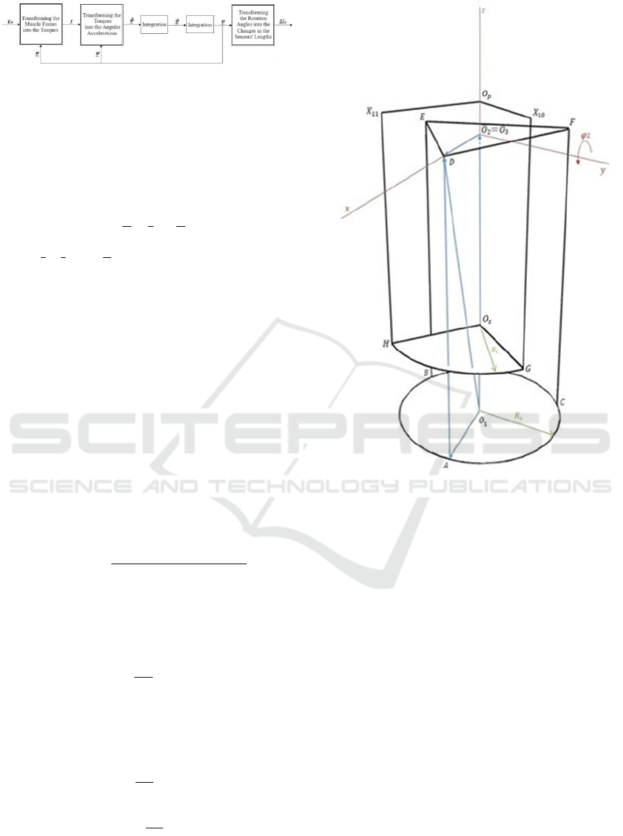
Figure 5: The block diagrams of the whole MIMO system
model.
3.1.1 Transforming the Muscle Forces into
the Toques
Based on the physical laws of angular rotation, the
corresponding torques can be calculated as follows
τ
= r × F ,
where τ , r and F represent the resulting torques
matrix, the distance vector and the muscles forces
matrix, respectively. Figure 6 shows the simplified
model of the robot hand axes in which the related
vectors to calculate the first muscle vector are shown
in blue.
The step-by-step calculations to get the first
muscle vector are as follows
1
𝑟⃗
D 3
=
13
T .
3
𝑟⃗
D 3 ,
1
𝑟⃗
D 1
=
1
𝑟⃗
3 1
+
1
𝑟⃗
D 3 ,
1
𝑟⃗
D A
=
1
𝑟⃗
D 1
-
1
𝑟⃗
A 1 .
If the coordinates of the first muscle force vector
1
𝑟⃗
D A
along x- , y- and z-axis are considered
𝑟
,
,𝑟
,
, and 𝑟
,
, respectively, the whole length
of 𝑟⃗
DA
can be stated as
𝑙
D A
=

𝑟
,

+𝑟
,

+𝑟
,

.
Therefore, the unit vector of the first muscle
force vector in the first coordinate system can be
expressed as
1
𝑒
D A
=



.
1
𝑟⃗
D A
.
Similarly, the unit vector of the second and third
muscle vector in the first coordinate system can be
determined by the following equations
1
𝑒
EB
=



.
1
𝑟⃗
EB
,
1
𝑒
FC
=



.
1
𝑟⃗
FC
.
Figure 6: The simplified system model to calculate the first
muscle vector, 𝑟⃗
D A
.
To correctly show the pulling direction of the
muscle forces, the unit matrices must be multiplied by
-1, resulting in the following vector
1
𝐹
⃗
M 1
= - F
M 1
.
1
𝑒
D A
,
where F
M 1
denotes the scalar value of the produced
forces of the first pneumatic muscle.
To simplify the further calculations, the related
vectors must be brought into the third coordinate
system, therefore
3
𝐹
⃗
M 1
=
13
T
-1
.
1
𝐹
⃗
M 1
,
Consequently, based on the equation (7) the
produced torque of the first muscle can be calculated
as follows
3
𝜏⃗
1
=
3
𝑟⃗
1
×
3
𝐹
⃗
M 1
,
The corresponding vectors of the second and the
third muscles can be calculated similarly. As a result,
(8)
(9)
(10)
(11)
(12)
(13)
(14)
(15)
(16)
(17)
(7)
ICINCO 2024 - 21st International Conference on Informatics in Control, Automation and Robotics
240

the aggregate torque can be stated as
∑ τ =
3
𝜏⃗
1 +
3
𝜏⃗
2 +
3
𝜏⃗
3
.
3.1.2 Transforming the Torques into the
Angles
According to the physical laws of rotation, the
relationship between the angular velocity and the
corresponding torque stated as
∑ τ = J
⋅ 𝜑 ,
where J denotes the moment of inertia of the mass to
which the torque has been applied. Therefore, the
angular velocity can be stated as
𝜑 = J
-1
. ∑ τ .
In order to calculate J, the top plate is considered
a triangular prism. The detailed calculations can be
found in (Mirafzal, 2023).
Correspondingly, the matrix of the rotation
angles can be calculated easily by two consecutive
integrator blocks in Simulink.
3.1.3 Transforming the Angles into the
Changes in the Sensors' Lengths
To calculate the sensors' lengths change, each of the
corresponding sensor vectors must be calculated
separately. Figure 7 shows the simplified model of the
robot hand axes in which the related vectors to
calculate the X
11
sensor vector are shown in blue.
Consequently, the
X
11
sensor vector, 𝑟⃗
11H
, can be
calculated by the following equations.
1
𝑟⃗
11 3
=
13
T .
3
𝑟⃗
11 3
,
1
𝑟⃗
11 1
=
1
𝑟⃗
3 1
+
1
𝑟⃗
11 3
,
1
𝑟⃗
11 S
=
1
𝑟⃗
11 1
-
1
𝑟⃗
S 1
,
1
𝑟⃗
11 H
=
1
𝑟⃗
11 S
-
1
𝑟⃗
H S
.
As a result, the length of the X
11
sensor can be
stated as
𝑙
X 11
=

𝑟
,

+𝑟
,

+𝑟
,

.
Accordingly, if the initial sensor length is
considered 𝑙
s0,
the length change of the X
11
sensor
can be stated as
𝛥𝑙
X 11
= 𝑙
X 11
- 𝑙
s 0
.
Figure 7: The simplified system model to calculate the X
11
sensor vector, 𝒓

⃗
11H
.
A similar approach can be followed to calculate
the length change of the X
10
sensor, 𝛥𝑙
X 10
.
3.2 Design of the Nonlinear Inverse
System Model
As shortly discussed previously, it is necessary to
design an inverse system model to complete the
flatness-based control block diagram. As the first
inverse block, the output values for the changes in the
sensors’ lengths, 𝛥𝑙
X 11
and 𝛥𝑙
X 10
, must be converted
into the corresponding rotation angle values, 𝜑
1
and
𝜑
2
. These output rotation angles as well as the desired
rotation angles are the inputs of the first flatness-
based angle controller, which is explained in more
detail in section 4. Figure 8 shows the schematic
block diagrams of the whole inverse system model.
(18)
(19)
(20)
(21)
(22)
(23)
(24)
(25)
(26)
Nonlinear Control and State Estimation for the Hand Axes of a Pneumatic Robot
241

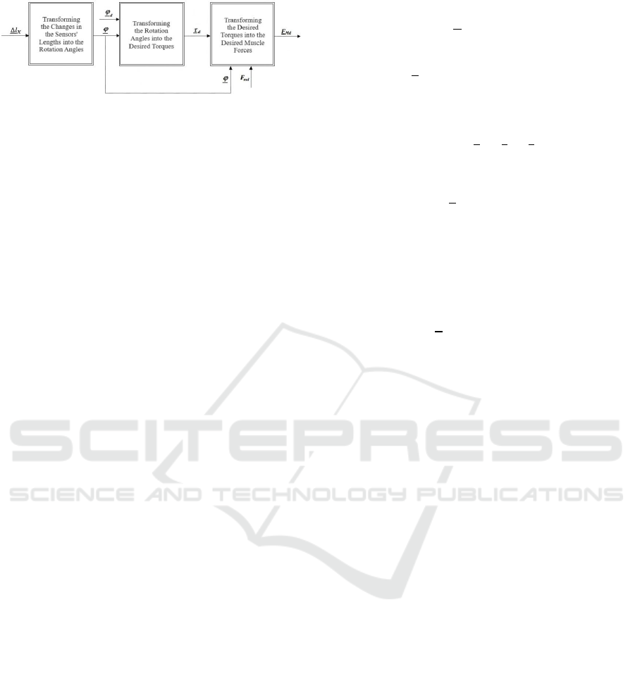
Figure 8: The block diagrams of the whole inverse system
model, in which 𝜑
d
, 𝜏

, 𝐹

, and 𝐹

represent the desired
rotation angle, torque, mean force, and muscle force,
respectively.
3.2.1 Transforming the Changes in the
Sensors’ Lengths into the Rotation
Angles
Although the changes in the sensors’ lengths can be
analytically calculated from the rotation angles in the
MIMO system model, the rotation angles cannot be
calculated analytically by the MATLAB “solve”
function, due to the complexity of the nonlinear
inverse model to calculate the angles. Therefore, a
lookup table is employed in Simulink to output the
rotation angles from the inputs, which are the changes
in the sensors’ lengths, numerically.
3.2.2 Transforming the Rotation Angles into
the Desired Torques
Given the rotation angles, that result from the lookup
table, the desired torques can be outputted. To do this,
the designed angle controller, which is described in
the equation (32) in section 4, must take the rotation
angles from the lookup table, as well as the desired
angles, that can be chosen by considering the system
limitations. Next, the controller outputs the second
derivative of the rotation angles, as the controlled
values. Then, the desired torques can be calculated,
having the moment of inertia, as described in the
equation (33) in section 4.
3.2.3 Transforming the Desired Torques
into the Desired Muscle Forces
The conversion of the desired torques to the desired
muscle forces could be challenging, due to the
complex nonlinear structure of the equations.
Nevertheless, by using an innovative approach, the
problem is solved completely analytically.
Due to the fact that the coefficients of the desired
muscle forces,
F
M1
, F
M2
and F
M3
, can be totally
separated from the muscle forces in the matrix of the
desired torques, the desired torques matrix can be
rewritten as follows
A
f
∙ F
Md
= 
𝜏

𝜏

𝐹

 ,
where
A
f
and F
Md
can be written as
A
f
= 
𝑎

𝑏

𝑐

𝑑

𝑒

𝑓







 ,
F
Md
= 
𝐹

𝐹

𝐹
,
 ,
and 𝐹

denotes the desired mean muscle force.
As a result, the desired muscle force matrix can be
calculated by
F
Md
= A
f
-1
∙ 
𝜏

𝜏

𝐹

 .
The desired muscle forces are used as the
reference values for the flatness-based force
controller, which is discussed in section 4.
4 SYSTEM ANALYSIS AND
DESIGN OF A NONLINEAR
TRAJECTORY TRACKING
CONTROL
Flatness-based control is a method that offers a cost-
effective and straightforward approach for nonlinear
models, enabling easy tracking of desired inputs with
the inclusion of feedforward as a compensator.
The general formula to design a flatness-based
controller can be stated as (Lévine, 2009)
𝜈=𝑦

(

)
+𝑎

𝑦

(

)
−𝑦

(

)



,
where 𝜈 denotes the control input to the system, 𝑦

represents the desired flat output or the reference
trajectory, 𝑎

refers to the feedback coefficient
ensuring stability (typically chosen to form a Hurwitz
polynomial), and n is the relative degree of the
system.
This approach effectively controls angles and
muscle forces (or pressures) and is implemented in
the control system, detailed in this section.
(27)
(28)
(29)
(30)
(31)
ICINCO 2024 - 21st International Conference on Informatics in Control, Automation and Robotics
242

4.1 Design of the Flatness-based Angle
Controller
The angles 𝜑
1
and 𝜑
2
are determined using sensor
feedback and the relationship between its length
change to the other components of the robot by means
of the vector-based modeling. Using numerical
methods, including lookup tables in
MATLAB/Simulink, sensor data can be converted
into controlled outputs.
For systems suitable for flatness-based control,
like this system, the design is straightforward. As the
relative degree of the angels in the system is 2,
according to equation (31), the control equations for
the main joint angles can be stated as
𝜑
i
= 𝜑
id
+ 𝑎

. (𝜑
id
– 𝜑
i
) + 𝑎

. (𝜑
id
– 𝜑
i
) .
Here, i={1, 2} for each of the angles and 𝜑
id
is the
desired angular acceleration, also acting as the
feedforward compensator, while 𝑎

and 𝑎

are
positive constants ensuring system stability.
Desired angle trajectories, e.g. varying sine
functions, can be freely chosen within physical
constraints, detailed further in section 5.
Next, torques are computed from the angular
accelerations, which are used to calculate total
torques about x- and y-axes

𝜏

𝜏

=
𝐽

𝐽

𝐽

𝐽

 . 
𝜑

𝜑

 ,
where 𝐽 denotes the moment of inertia of the mass at
the top of the robot hands to which the torques have
been applied, that has been approximated by a
triangular prism. This process is implemented in the
angle controller.
4.2 Design of the Flatness-based Force
Controller of the Pneumatic
Muscles
In addition to rotation angles, it is crucial to control
the pneumatic muscle forces through a separate
tracking controller.
The muscle force 𝐹

comprises the static force
𝐹
,
and the hysteresis force 𝐹
,
, with the latter
being negligible, as written in equation (4) in section
2.
As mentioned earlier, the static force is calculated
using coefficients 𝑎

and 𝑏

determined via the
Recursive Least Squares (RLS) method, as described
in section 2, equations (5) and (6). The derivative of
muscle pressure 𝑝
Mi
is expressed as (Schindele et al.,
2013)
𝑝
Mi
=



 




𝑅

𝑇

𝑚

−








𝑧

𝑝


=𝑘

(
Δ𝑙

,𝑝

)
𝑚

− 𝑘

Δ𝑙

,Δ𝑙


,𝑝

 𝑝

,
where i = {1, 2, 3}, 𝑉

denotes the volume of the
pneumatic
muscles, R
L
= 287 the air gas constant,
n = 1.26
the identified polytropic exponent,
T
Mi
= 294 K the internal temperature, and Δ𝑙

the
contraction length.
The volume of the pneumatic muscles 𝑉

is
defined as
𝑉

(
Δ𝑙

,𝑝

)
=𝑎

Δ𝑙


 𝑝



+  𝑏

Δ𝑙


,


where the coefficients 𝑎

and 𝑏

can be identified
experimentally, just like the polynomial function of
the muscle forces.
The mass flow rate 𝑚

is given by:
𝑚

=











 








,
where 𝑓

and 𝑓

are derived from the equation (6).
By considering 𝜈

=𝐹


, similar to designing the
angle controller based on equation (31), and
considering that the relative degree of the muscle
forces in the system is 1, the flatness-based force
controller can be formulated as
𝐹


=𝐹


+𝑎

.
(
𝐹

− 𝐹

)
.
Here, i={1, 2, 3} for each of the muscles, and 𝐹


act as the feedforward compensator, while 𝑎

must be
chosen positive to ensure the system stability.
5 DETERMINATION OF THE
DESIRED TRAJECTORIES
The robot pneumatic system has restrictions such as
the rotation angles, 𝜑
1
and 𝜑
2
, of the main joint and
the maximum pressure from the pneumatic control
unit (PCU), due to its physical characteristics. These
(32)
(33)
(34)
(36)
(37)
(35)
Nonlinear Control and State Estimation for the Hand Axes of a Pneumatic Robot
243

limitations must be incorporated into the model for
realism. Typically, a target polynomial is used for the
desired angles to improve control response and
derivatives (Mirafzal, 2023). This section details
these system restrictions, methods, and resulting
trajectories.
5.1 Minimum Force/Pressure
Requirements
The pulling force of the pneumatic muscles is limited
by the compressed air pressure. The initial pressure is
approximately 1 bar, while the laboratory maximum
is 8 bars due to the pneumatic control unit's
constraints. Additionally, the muscle forces have
minimum and maximum limits. Tests showed that the
desired mean force, F
m
, should not fall below 15
newtons, as lower values result in unrealistic negative
forces. Consequently, the maximum forces and
torques are functions of the compressed air pressure,
which is capped at 8 bars, limiting the corresponding
forces and torques.
5.2 Feasible Trajectories for the end
Effector Rotation Angles
The primary constraints of the pneumatic robot
system include the feasible rotation angles due to
physical limitations. Rotations about the z-axis are
not allowed, and rotations about the x- and y-axes are
limited and cannot approach e.g. 90 degrees. Not all
combinations of the main angles, 𝜑
1
and 𝜑
2
, are
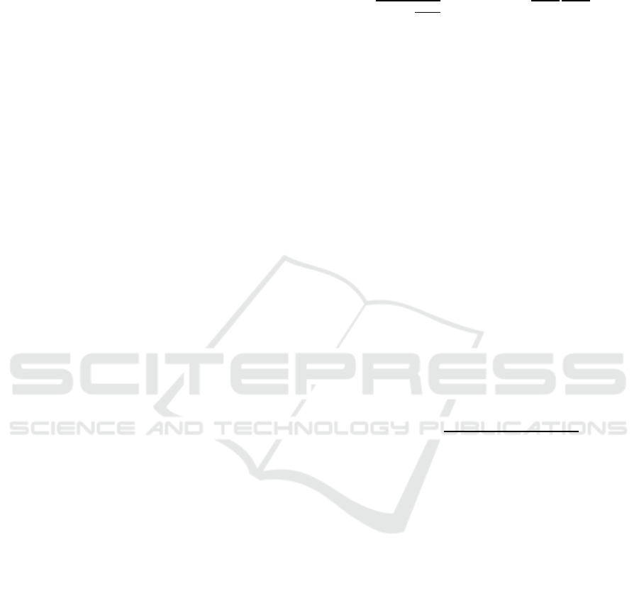
practically achievable. Practical trajectory plots for
the changes in the sensors’ length are created in the
laboratory to determine the possible angles from 1377
different states, as shown in figure 9.
Figure 9: The possible trajectories for the changes in the X
10
and X
11
sensors’ lengths that are measured practically in the
laboratory for 1377 reachable points.
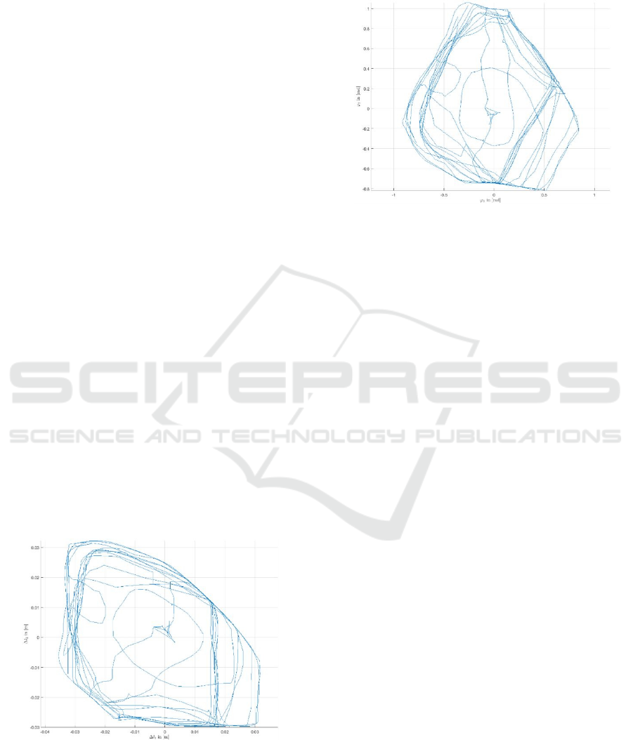
As a result, the corresponding 𝜑
1
and 𝜑
2
angles
can be plotted using MATLAB, as shown in figure
10.
Figure 10: The corresponding trajectories for the main
angles for all of the 1377 measured points resulting from
the sensors data.
Some maximum points in Figure 10 are achieved
manually, not through full compressed air pressure,
indicating some unreachable points. In addition, the
plot should be symmetric, due to the symmetric
structure of the system, revealing missing points.
6 ESTIMATION OF THE STATE
AND DISTURBANCE
In advanced control systems, feedback alone is often
insufficient for achieving quick and accurate
responses due to errors, noise, and disturbances.
Feedback compares current outputs with set points to
identify errors but compensates only after errors
occur, leading to potential delays. In addition to
feedback, two main compensators, including
feedforward and observer (estimator), are typically
employed to address the mentioned issues.
Feedforward, as explained briefly in the flatness-
based control design, anticipates errors using prior
knowledge of disturbances, compensating before
errors are detected by feedback. Furthermore, the
observer, or estimator, is used when employing
sensors is impractical or costly, as it estimates system
states and reduces noise and cost, making it essential
for complex systems where direct measurement is
impossible. These strategies work together to enhance
error correction and improve system performance.
The system model described earlier is idealized
and does not account for real-world disturbances,
particularly friction, which significantly affects
ICINCO 2024 - 21st International Conference on Informatics in Control, Automation and Robotics
244

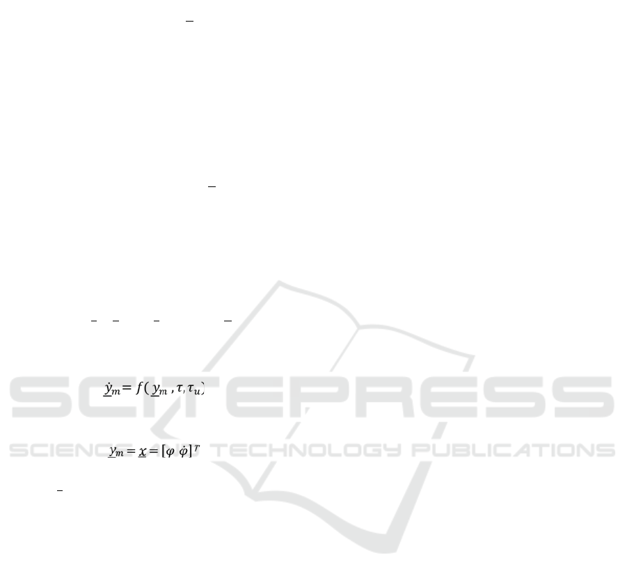
mechanical systems. The nonlinear friction model for
such systems can be expressed as (Mirafzal, 2023)
𝜏

=𝜏

.𝑡𝑎𝑛ℎ





,
where 𝜏

denotes the nonlinear friction, 𝜏

and ε are
constants, with ε typically set to a small value, such
as 0.01, based on experience. Damping, especially
speed-proportional damping, also affects the system
and is represented as b. 𝜑, where b is a constant
relating angular velocity to friction.
Thus, the total friction torque can be stated as
𝜏

= 𝑏.𝜑+ 𝜏

.𝑡𝑎𝑛ℎ





.
In this experiment, the constants are considered
b = 0.1, 𝜏

= 0.0015, and 𝜀= 0.01 The state space
representation for the torque about each rotation axis
is given by

𝜑
𝜑
 = 
𝜑


−


𝜑−


𝜏

.𝑡𝑎𝑛ℎ





 ,
where
,
and
.
Here, y
m
refers to the state vector. Equation (40)
can be applied separately to each rotation angle,
𝜑

and 𝜑

, with 𝜏 representing the torque about the x-
and y-axes, respectively.
Therefore, this friction will be estimated and used
as a compensator in the control system model.
In this system model, various states, such as the
main angles of the central joint, can be estimated.
However, compensating friction disturbances has
higher priority. Given that friction influences the
aggregate torques and the model uses a linear
approach for these calculations, the Kalman Filter can
estimate friction in this system (Welch et al., 2006).
Consequently, it is employed to estimate the
disturbance torque attributed to friction. The detailed
design of the Kalman Filter can be found in (Mirafzal,
2023).
The next section will compare the estimation
results with the noisy model disturbance torque and
analyze the overall model control response.
7 SIMULATIVE
INVESTIGATION AND
EVALUATION
To evaluate the control system’s response,
adjustments are made to simulate real-world
conditions with disturbances, noise, and initial
conditions. Potentiometers and pressure sensors
received noise with specified variances. System limits
and delays are also set. Friction is estimated and
compensated using a Kalman Filter.
The system's response is evaluated against desired
trajectories for both angles and muscle forces. The
next step is to tune the controllers to receive a
satisfactory response of the system. Effective tuning
of flatness-based controllers is achieved by adjusting
coefficients iteratively. To adjust the coefficients of
the controllers, the eigenvalues should be chosen for
each controller. Through multiple rounds of trial and
error and examining how well the outputs can track
the desired trajectories in Simulink, the eigenvalues
of -225 and -1100 are chosen for the angle controller
and the force controller, respectively. As a result, the
characteristic polynomial for the angle controller can
be stated as
𝑃(𝑆)=(𝑆 + 225)

=𝑆

+ 450 𝑆+ 50625 .
Therefore, the coefficients of the flatness-based
angle controller in equation (32) can be chosen as
𝑎

= 50625 and 𝑎

= 450.
Similarly, the characteristic polynomial for the
force controller can be stated as
𝑃
(
𝑆
)
=𝑆+ 1100 .
As a result, the coefficient of the flatness-based
force controller in equation (37) can be chosen as
𝑎

= 1100.
After implementation of the selected control
coefficients, the tracking behavior of the system
shows high accuracy and fast response to the desired
trajectories.
Figures 11 and 12 show the tracking behavior of
the system as a response to the desired sine wave
trajectories. Figure 13 also illustrates how well the
Kalman Filter estimates the friction torques.
(38)
(39)
(40)
(43)
(44)
(41)
(42)
Nonlinear Control and State Estimation for the Hand Axes of a Pneumatic Robot
245

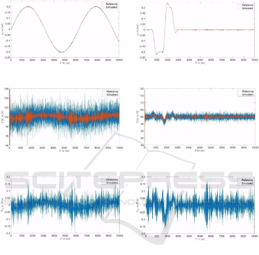
Figure 11: The output of the second angle, 𝜑
2,
compared to
sample reference sine wave trajectories.
Figure 12: The output of the third muscle force, F
M3
,
compared to the reference values.
Figure 13: The estimated friction torque about y-axis
compared to the reference values.
Similarly, figures 14 and 15 illustrate how well
the system follows more complex desired trajectories
for the first rotation angle and the third muscle force,
respectively, demonstrating effective control despite
assumed disturbances. The Kalman Filter also
effectively estimates friction torques, as shown in
Figures 16, aligning closely with real values under
various conditions.
Overall, the simulation results validate the proper
determination of the physical conditions, as well as
the suitability of the controller designs and the
coefficient selections, ensuring the system performs
well under different operating conditions, in which
factors such as friction torque play important roles in
the system’s response.
Figure 14: The output of the first angle, 𝜑
1,
compared to
sample reference trajectories.
Figure 15: The output of the third muscle force, F
M3
,
compared to the reference values.
Figure 16: The estimated friction torque about y-axis
compared to the reference values.
8 CONCLUSIONS
This experiment focuses on modeling and controlling
a pneumatic robot hand axes system, with a key
emphasis on central joint rotation angles and
pneumatic muscle forces. Using transformation
matrices simplifies kinematic relationships, while
Recursive Least Squares helps characterize
pneumatic muscle behavior.
A flatness-based control approach is chosen for its
ability to effectively track desired trajectories despite
system non-linearities.
ICINCO 2024 - 21st International Conference on Informatics in Control, Automation and Robotics
246

To enhance realism, disturbances like friction
torques and sensor noise are introduced and mitigated
using a Kalman Filter observer. Tuning controller
coefficients through iterative testing optimizes
system response, ensuring outputs closely matches
desired values.
In conclusion, this research demonstrates the
practicality and efficiency of pneumatic actuators in
generating substantial forces, supported by robust
flatness-based controllers. Future work could explore
alternative actuators and control strategies like the
Backstepping or the Sliding-Mode-Control for
further system enhancement.
REFERENCES
Daerden, F., and Lefeber, D. (2002). Pneumatic artificial
muscles: Actuators for robotics and automation.
European Journal of Mechanical and Environmental
Engineering, Vol. 47, No. 1, pages 11–22.
Deaconescu, T., and Deaconescu, A. (2016). Study
Concerning the Hysteresis of Pneumatic Muscles,
Applied Mechanics and Materials, Trans Tech
Publications, Switzerland. Vol. 841, pages 209-214.
Franklin, Powell, and Emami-Naeini. (2019). Feedback
Control of Dynamic Systems, Pearson. 8th edition.
Lévine, J. (2009). Analysis and Control of Nonlinear
Systems: A Flatness-based Approach, Springer.
Mirafzal, S. H. (2023). Nonlinear Control and State
Estimation for the Hand Axes of a Pneumatic Robot.
Master’s thesis at the Faculty of Mechanical
Engineering and Ship Technology, University of
Rostock.
Schindele, D., and Aschemann, H. (2013). Comparison of
Cascaded Backstepping Control Approaches with
Hysteresis Compensation for a Linear Axis with
Pneumatic Muscles. IFAC, Vol. 46, No. 23, pages 773-
778.
Vo, T. M., Kamers, Ramon, H., and Van Brussel, H. (2010).
Characterization of Hysteresis in a Pneumatic Muscle
Manipulator with Accounting for the Creep Effect,
IFAC, Vol. 43, No. 21, pages 296-302.
Welch, G., and Bishop, G. (2006). An Introduction to the
Kalman Filter. Department of Computer Science,
University of North Carolina at Chapel Hill.
Woernle, C. (2016). Mehrkörpersysteme. Eine Einführung
in die Kinematik und Dynamik von Systemen starrer
Körper, Springer-Vieweg. Wiesbaden. 2
nd
edition.
Xie, L., Yang, H., and Ding, F. (2011). Recursive least
squares parameter estimation for non-uniformly
sampled systems based on the data filtering.
Mathematical and Computer Modelling No. 54, pages
315–324.
Nonlinear Control and State Estimation for the Hand Axes of a Pneumatic Robot
247