Red Wine Prediction Comparing Several Machine Learning Models
Yitong Huang
Chemical Engineering and Bioengineering College, Zhejiang University, Hangzhou, China
Keywords: Machine Learning, Red Wine Quality Prediction, Optimization.
Abstract: With the increasing interest in red wine among consumers, the quality of red wine has become a topic of
significant importance. However, the limited availability of trained wine tasters in certain regions, especially
for red wine, has hindered the progress of the red wine industry. Therefore, the utilization of mathematical
models and computer software for assessing the quality, identification, and classification of red wine is crucial.
The research articles primarily focus on comparing the accuracy of various methods such as Random Forest,
Radial Basis Function, and Naive Bayes models. Among these models, the Random Forest method
demonstrates the highest accuracy, with an adjusted of 0.8656. The study also investigates the factors
influencing the model's accuracy and proposes optimization strategies using NBF_NB and Genetic algorithms
for enhanced precision in the results. As the demand for high-quality red wine continues to grow, the
implementation of advanced analytical techniques and optimization methods is imperative for ensuring
accurate and efficient wine quality evaluation.
1. INTRODUCTION
Red wine is an alcoholic product with a long history
and profound cultural heritage. The quality of red
wine has a crucial impact on consumer experience,
the reputation of production companies and market
competitiveness. Therefore, predicting the quality of
red wine has become one of the focuses of the wine
making industry and consumers. Red wine quality
evaluation method is an important aspect in the field
of red wine research because it is directly related to
consumers' perception and choice of red wine (Pei,
2022). To forecast the red wine quality, many efforts
have been made to consider miscellaneous factors
affecting it.
Machine learning research aims to tackle
challenges in time by dividing them into accessible
parts and addressing them individually through
machine learning algorithms. For this research Dahal
et al. utilized diverse machine learning techniques to
identify key features that influence wine quality (Pei,
2022). The study conducted by the researchers
utilized 11 physiochemical attributes creating
machine learning models aimed at the red wine
quality prediction (Dahal et al., 2021). Kumar and
colleagues applied data mining techniques for
extracting insights on the datasets provided by the
UCL (Kumar et al., 2020). Trivedi and Sehrawat
compared various classification algorithms,
elucidating the reasons behind the varying accuracies
produced by different algorithms (Trivedi and
Sehrawat, 2018). A decision tree classifier is used to
determine the red wine by Lee et al., whereas Mahima
Gupta and group combined and used Random Forest
and K-Nearest Neighbors algorithms to categorize
wines as good, average, or poor (Lee et al., 2015 &
Mahima et al., 2020). The main objective of this
research endeavor aims to predict wine quality with
methodologies that encompass both physiochemical
and chemical attributes. Nonetheless, the project
encounters certain challenges. The foremost obstacle
lies in the limited sample size, a hurdle that the
researchers are striving to surmount in their studies.
Given the arduous and costly nature of gathering
extensive viticulture data, synthetic data resembling
the original dataset is generated to address this issue.
Another concern is the risk of data leakage, which
occurs when information is inadvertently shared
between datasets during the preprocessing phase of
program execution.
2. METHODOLOGIES
In this research, we first perform exploratory data
analysis on the dataset and preprocess the input data.
Huang, Y.
Red Wine Prediction Comparing Several Machine Learning Models.
DOI: 10.5220/0013007200004601
Paper published under CC license (CC BY-NC-ND 4.0)
In Proceedings of the 1st International Conference on Innovations in Applied Mathematics, Physics and Astronomy (IAMPA 2024), pages 169-173
ISBN: 978-989-758-722-1
Proceedings Copyright © 2024 by SCITEPRESS – Science and Technology Publications, Lda.
169

Then we construct and train several machine learning
models, including Radial basis function model(RBF),
naive Bays model(NBC), Random forest model, to
obtain corresponding results for further analysis.
RBF (Radial Basis Function):It is composed of J.
Moody and C The neural network algorithm based on
radial basis functions proposed by Darken in 1988.
RBF neural network is a local approximation network
that can approximate any continuous or discrete
function with arbitrary accuracy (Bi et al., 2016), and
can handle rules that are difficult to analyze within
the system. It is quite effective when handle nonlinear
classification and prediction problems.
Three layer consist the neural network and
function, they are input layer, hidden layer, and
output layer. The input layer is the same as other
neural network, in the article, the input layer
represents physical and chemical test characteristic
attributes of red wine, the datasets score the
characteristic attributes of the red wine, resulting in
the confirmation for the final quality prediction. the
Its structural diagram is shown in Figure 1. As shown
in the below figure, the input layer is (X1, X2,..., Xp),
the hidden layer is (c1, c2,..., ch), and the output layer
is y, and (w1, w2,..., wm) represents the hidden layer
to the classification of red wine quality grades (Bi et
al., 2016). The output layer’s connection weights are
determined by a nonlinear function, h(x), known as a
radial basis function, utilized by each node in the
hidden layer. The primary function of the hidden
layer is to transform the vector containing low-
dimensional statistical data, p, into a high-
dimensional representation, h, which ultimately
influences the quality assessment. This
transformation enables the network to address cases
of linear inseparability in low dimensions by making
them separable in higher dimensions.
The central concept driving this process is the
kernel function, which ensures that the mapping from
input to output within the network is nonlinear, while
maintaining linearity in the network’s output with
adjustable parameters. By solving the network’s
weights directly through linear equations, the learning
process is significantly accelerated, and the risk of
getting stuck in local minima is minimized. The
activation function of a radial basis function neural
network is typically represented by a Gaussian
function.
R(x

−c

)=exp(−

ơ

||x

−c

||

) (1)
The structure of radial basis neural networks can
be obtained as follows:
𝑦

=
∑
𝜔



𝑒𝑥𝑝(−

ơ

||𝑥

−𝑐

||

)+𝑏

j=1,2,...,n
(2)
Among them, xp is the p-th input sample, ci is the
i-th center point, and h is the number of nodes in the
hidden layer. N is the number of samples or
classification outputs, and bi is the threshold of the i-
th neuron.
NBC: Naive Bayes classifier (NBC) is a very
simple classification algorithm. For the red wine
quality to be classified, under the condition of the
event occurring, the probability of occurrence for
each category is the highest, indicating which
category it is considered to belong to (Liang, 2019).
The NBC model assumes that attributes are
independent of each other, but in real data, each
attribute is correlated, which is precisely this
assumption that limits the use of the NBC model.
Bayesian method can be calculated by assuming a
prior probability and the conditional probability
obtained from observation data under a given
assumption:
P(O|) =
(|)()
()
(3)
Assuming that each data sample Y={y1, y2,..., yn}
yis a set of n-dimensional vectors with n class labels
C C C n, 1, 2.
Obtaining:
max{P(x=𝐶

|Y),P(y=𝐶

|Y),...,y=𝐶

|Y)} (4)
Transform the classification problem into a
conditional probability problem, where P (Y) is
constant for all classes, so the probability of each C
classification occurring under the condition of Yis P
(C | Y). Then, take the C at the maximum probability
as our answer and determine the class label Ci.
Because X, as a sample data, often has a large
dimension, probability of any combination of features
is usually difficult to analysis, which requires the use
of the word "naive" in naive Bayes. Assuming that the
conditions are independent of each other, the number
of parameters to be solved is greatly reduced. Only
one P (X | C) needs to be solved separately, and then
multiplied to obtain: while the prior probability can
be obtained from the training sample:
P(X|𝐶

)=
∏
𝑃(


𝑥

|𝐶

) (5)
The prior probability can be obtained from the
training samples:
P(𝐶

)=



(6)
IAMPA 2024 - International Conference on Innovations in Applied Mathematics, Physics and Astronomy
170

Among them, the total number for training
samples is the numerator, and the whole number of
samples is the denominator.
Random forest: Multiple decision trees is
combined to apply the ensemble learning, that is
called Random forest. Each decision tree serves as a
base unit in this algorithm, which falls under the
umbrella of ensemble learning methods. Intuitively,
each decision tree functions as a classifier,
particularly in scenarios involving classification tasks.
When presented with an input sample, the ensemble
of N trees generates N classification outcomes. The
random forest algorithm then consolidates these
individual classification results by aggregating the
votes and selecting the category with the highest
number of votes as the final output. This approach
essentially embodies the Bagging concept. The
motivation behind the development of random forests
stems from the limitations of decision trees, which
exhibit weak generalization capabilities due to their
singular decision path. By leveraging random forests,
these shortcomings can be effectively addressed, as
the ensemble of decision trees collectively enhances
the algorithm’s generalization performance (Cao et
al., 2022).
3. RESULT AND DISCUSSION
The relevant research mentioned in the articles bases
on the application of jupyterlab, the predictive
classification based on characteristic data of wine
prediction.
The main task of the research is to extract data
from the database, remove blank or missing rows, and
retrieve relevant model data packages to predict and
classify the remaining feature data related to red wine
prediction
This paper focuses on the datasets provided in
UCI of the red wine quality.
The datasets contains 11 physical and chemical
test characteristic attributes, The 12th column is the
quality evaluation score of the wine, ranging from 0
to 10. And the work is to predict the quality
evaluation using those 11 characteristic (Ma, 2022).
The preparation work includes deleting rows with
missing values, converting all data to numeric data,
because the data set most distributes in six grades 3-8
(Liu, 2019), the articles mainly divide those datasets
into six categories (Table 1).
3.1. Evaluation metrics
 Mean Absolute Percentage Error (MAPE)
MAPE provides the error in terms of percentages,
the smaller the MAPE the better the predictions.
 Adjusted
2
R
Both R-squared and adjusted R-squared indicate
the proportion of variance in a dependent variable that
can be accounted for by independent variables within
a regression model. However, adjusted R-squared
serves as an evaluation of how successful a regression
model predicts responses for new observations. It will
increase when more useful variables are added to the
model, and decrease reversely (Wu and Yang, 2022).
3.2. Discussion
To improve the classification accuracy of red
wine quality grade, a machine learning theory
combining RBF neural network and naive
Bayesian classification is used to construct a
classification model based on the determination
of multiple physical and chemical components
extracted from red wine, achieving effective
classification of red
wine quality. This model is still
based on the RBF, but when confirming the basis
connection between the hidden layer and the output
layer, naive Bayes model could be used so the basis
connection would be more accurate. This
combination is really effective especially when there
is a myriad of statistics (Table 2).
Table 1: Datasets of wine.
Fixed
acidity
Volatilc
acidity
Citric
acid
Residual
sugar
chiorides
Free
Sulfur
dioxide
Total
Sulfur
dioxide
density PH sulphates alcohol quality
0 7.4 0.70 0 1.9 0.076 11.0 34.0 0.9978 3.51 0.56 9.4 5
1 7.8 0.88 0 2.6 0.098 25.0 67.0 0.9968 3.20 0.68 9.8 5
2 7.8 0.76 0.04 2.3 0.092 15.0 54.0 0.9970 3.26 0.65 9.8 5
Red Wine Prediction Comparing Several Machine Learning Models
171

Table 2 Result of evaluation.
Model MAPE
Adjusted
2
R
RBF 0.3287 0.809375
NBC 0.3160 0.815626
RF 0.3098 0.865625
NBF_NB 0.3032 0.871875
It is shown that the improved algorithm
combining the two models enhanced the
classification accuracy of quality levels obviously
comparing with separate model using; It has positive
practical reference value for red wine processing
enterprises.This indirectly confirms that in the face of
big data calculations with over a thousand data points
and eleven parameters in this study, the combination
of models will have more advantages.But the
optimization does now show apparent advantages
among the RF model.This probably because the RF
itself is proficient in dealing with high dimension and
large scale datasets, making it a reliable methods in
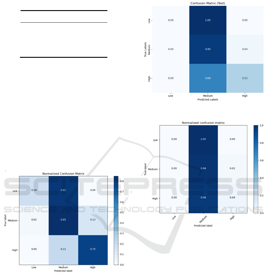
the research. Normalized Confusion Matrix about
three basic model are shown in figure 1, figure 2 and
figure3.
Figure 1: The confusion matrix of RBF
Figure 2: The confusion matrix of NBC
Figure 3: The confusion matrix of RF
4. CONCLUSION
In summary, this paper includes both machine
learning and some optimization to find a suitable
method to predict Red wine quality. These models are
RBF, NBC, RF as basic and NBF_NB as optimization.
Among all of these models, two optimization
obviously make the more accurate prediction, and the
classification effect is significant. All in all, after
using several effective methods to the training model,
classifiers’ performance successfully enhanced . The
significance of data generation algorithms and the
role of feature selection count most essentially in this
study. However, if further adjust the parameters of
those models, there might be more improvement. The
theory in the paper can be applied to intelligent
detection of food quality in other food processing
IAMPA 2024 - International Conference on Innovations in Applied Mathematics, Physics and Astronomy
172

industries, which has practical significance for some
food processing enterprises. With the continuous
deepening of learning in the field of machine learning,
more useful and efficient models can be developed
and widely applied.
REFERENCES
Pei Wenhua. Research on Red Wine Quality Classification
Based on Machine Learning. Science and Industry,
2022, 22(12): 304-309.
Dahal, K., Dahal, J., Banjade, H., & Gaire, S.. Prediction of
Wine Quality Using Machine Learning Algorithms.
Open Journal of Statistics, 2021, 11, 278-289.
S. Kumar, K. Agrawal, & N. Mandan. Red Wine Quality
Prediction Using Machine Learning Techniques. 2020
International Conference on Computer Communication
and Informatics (ICCCI), Coimbatore, India, 2020, pp.
1-6.
A. Trivedi & R. Sehrawat. Wine Quality Detection through
Machine Learning Algorithms. 2018 International
Conference on Recent Innovations in Electrical,
Electronics & Communication Engineering
(ICRIEECE), Bhubaneswar, India, 2018, pp. 1756-
1760.
S. Lee, J. Park, & K. Kang. Assessing wine quality using a
decision tree. 2015 IEEE International Symposium on
Systems Engineering (ISSE), Rome, Italy, 2015, pp.
176-178.
Mahima, Gupta, U., Patidar, Y., Agarwal, A., Singh, K.P.
Wine Quality Analysis Using Machine Learning
Algorithms. Micro-Electronics and
Telecommunication Engineering. Springer,
Singapore,2020.
Bi Yanliang, Ning Qian, Lei Yinjie, et al. Classification of
Wine Quality Levels Using Improved Genetic
Algorithm Optimized BP Neural Network. Computer
Measurement & Control, 2016, 24(01): 226-228.
Liang Shuqi. Red Wine Quality Prediction System Based
on Naive Bayes Principle. China High-Tech, 2019(01):
95-97.
Cao, Y., Chen, H., & Lin, B. Wine Type Classification
Using Random Forest Model. Highlights in Science,
Engineering and Technology, 2022, 4, 400-408.
Ma Dongjuan. Discriminant Analysis of Red Wine Quality
Based on Physical and Chemical Indicators of Grapes.
Modern Food, 2022, 28(24): 181-184.
Liu Pan. Classification of Red Grape Wine Quality Levels
Based on RBF and Naive Bayes. Electronic
Technology and Software Engineering, 2019(04): 144-
145.
X. Wu & B. Yang. Ensemble Learning Based Models for
House Price Prediction, Case Study: Miami, U.S. 2022
5th International Conference on Advanced Electronic
Materials, Computers and Software Engineering
(AEMCSE), Wuhan, China, 2022, pp. 449-458.
Red Wine Prediction Comparing Several Machine Learning Models
173