Finding Strong Lottery Ticket Networks with Genetic Algorithms

Philipp Altmann, Julian Sch

onberger, Maximilian Zorn and Thomas Gabor

LMU Munich, Germany

Keywords:

Evolutionary Algorithm, Neuroevolution, Lottery Ticket Hypothesis, Pruning, Neural Architecture Search.

Abstract:

According to the Strong Lottery Ticket Hypothesis, every sufﬁciently large neural network with randomly

initialized weights contains a sub-network which – still with its random weights – already performs as well

for a given task as the trained super-network. We present the ﬁrst approach based on a genetic algorithm to

ﬁnd such strong lottery ticket sub-networks without training or otherwise computing any gradient. We show

that, for smaller instances of binary classiﬁcation tasks, our evolutionary approach even produces smaller and

better-performing lottery ticket networks than the state-of-the-art approach using gradient information.

1 INTRODUCTION

A central aspect to the wide success of artiﬁcial neu-

ral networks (ANNs) is that they are usually designed

to be overparametrized (Aggarwal et al., 2018). That

means that they feature more parameters (weights)

than are strictly necessary to represent the function

they are meant to approximate. However, it is also

that overparametrization that constructs a solution

landscape that is friendly towards relatively simple

optimization strategies like stochastic gradient de-

scent (Shevchenko and Mondelli, 2020), whose ap-

plication is also enabled by the fact that neural net-

works are usually differentiable and can thus pro-

vide gradient information to the optimization algo-

rithm. The Lottery Ticket Hypothesis (Frankle and

Carbin, 2018) and its variants (Ramanujan et al.,

2020) have provided a different perspective on the

properties of neural networks: Among the randomly

initialized weights (before any optimization), some

weights have already “won the lottery” by being eas-

ily trainable. Furthermore, in any sufﬁciently over-

parametrized network, there already exist — at the

point of random initialization — certain subnetworks

that (when unhinged from the rest of the network) ap-

proximates the desired function as accurately as the

whole network would after optimization. Thus, if

these subnetworks or strong lottery tickets could be

found easily, the whole training process of neural net-

works could be skipped. Figure 1 illustrates a lottery

ticket network evolved from a full network with much

more active (i.e., non-zero) connections.

Finding such subnetworks naturally requires a

Figure 1: Illustration of a lottery ticket network. Top: Full

network graph. Red connections persist in most evolved lot-

tery ticket networks in an example population (blue connec-

tions do not). Bottom: Example of an evolved lottery ticket

subnetwork with only a fraction of active connections.

substantial computational load, as the number of pos-

sible combinations of connections to prune from the

subnetwork grows exponentially with the network

size. This makes it difﬁcult for a lottery-ticket-based

optimization alternative to succeed in practice. In

fact, state-of-the-art methods for ﬁnding lottery tick-

ets tend to utilize regular training steps of the full net-

work (without changing the weights) to identify more

important connections to be kept in the subnetwork.

This paper presents a novel approach to ﬁnd-

ing strong lottery tickets based purely on combina-

torial evolutionary optimization without training the

weights or utilizing gradient information. To the best

of our knowledge, this is the ﬁrst approach in this di-

rection. We summarize our contribution as follows:

• We show that a basic genetic algorithm (GA) can

already produce strong lottery ticket networks.

• Our approach yields sparser and more accurate

networks compared to the gradient-based state-of-

the-art in exemplary binary classiﬁcation tasks.

• Uncovering scenarios where the utilized GA op-

erations are insufﬁcient, we hope to pave the way

for further investigating the applicability of GAs

for optimizing neural networks or similar entities.

Altmann, P., Schönberger, J., Zorn, M. and Gabor, T.

Finding Strong Lottery Ticket Networ ks with Genetic Algorithms.

DOI: 10.5220/0013010300003837

Paper published under CC license (CC BY-NC-ND 4.0)

In Proceedings of the 16th International Joint Conference on Computational Intelligence (IJCCI 2024), pages 449-460

ISBN: 978-989-758-721-4; ISSN: 2184-3236

449

2 RELATED WORK

The Lottery Ticket Hypothesis has received consider-

able attention in recent years, and as such, many con-

nections to adjacent ﬁelds have been discovered. In

this section, we will elaborate on the existing litera-

ture and how it relates to our work.

Lottery Ticket Hypothesis. Frankle and Carbin

(2018) discovered that a network that was pruned af-

ter training and then had its remaining weights reset

to their original random-initialized value could then

be trained again to achieve a comparable test accu-

racy to the original network in a similar number of

iterations. They called this phenomenon the Lottery

Ticket Hypothesis (LTH) and the pruned subnetwork

a winning ticket. They developed an algorithm based

on iterative magnitude pruning to ﬁnd these winning

tickets. Since then, many approaches have been de-

veloped to ﬁnd these winning tickets: Jackson et al.

(2023) use an evolutionary algorithm where they cal-

culate the ﬁtness based on the network density and

validation loss in an attempt to deal with the trade-

off between the sparsity and the accuracy of the sub-

network. Other subsequent work (Zhou et al., 2019;

Wang et al., 2020b) extended the LTH by empiri-

cally showing that it is possible to ﬁnd subnetworks

that already have better accuracy than random guess-

ing within randomly initialized networks without any

training. Zhou et al. (2019) identify neural network

masking as an alternative form of training and intro-

duce the notion of “supermasks.”

Strong Lottery Ticket Hypothesis. Ramanujan

et al. (2020) built upon this idea and proposed the

Strong Lottery Ticket Hypothesis (SLTH): A sufﬁ-

ciently overparameterized neural network with ran-

dom initialization contains a subnetwork, the strong

lottery ticket (SLT), that achieves competitive accu-

racy (w.r.t. the large, trained network) without any

training (Malach et al., 2020). Additionally, they in-

troduced edge-popup, an algorithm for ﬁnding strong

lottery tickets by approximating the gradient of a so-

called pop-up score for every network weight. These

popup scores are then updated via stochastic gra-

dient descent (SGD). A series of theoretical works

studied the degree of required overparameterization

(Malach et al., 2020; Orseau et al., 2020; Pensia

et al., 2020) and proved that a logarithmic overparam-

eterization is already sufﬁcient (Orseau et al., 2020;

Pensia et al., 2020). On the quest for more efﬁ-

cient methods for ﬁnding SLTs, Whitaker (2022) pro-

posed three theoretical quantum algorithms that are

based on edge-popup, knowledge distillation (Hinton

et al., 2015), and NK Echo State Networks (Whit-

ley et al., 2015). Finally, Chen et al. (2021) intro-

duced an additional type of high-performing subnet-

work called “disguised subnetworks” that differ from

regular SLTSs in the way that they ﬁrst need to be

“unmasked” through certain weight transformations.

They retrieve these special subnetworks via a two-

step algorithm performing sign ﬂips on the weights of

pruned networks using Synﬂow (Tanaka et al., 2020).

Weak Lottery Ticket Hypothesis. Only a few

methods for ﬁnding strong lottery tickets have been

developed to this point, and most of the empirical

work has been focused on the original LTH. They

identify so-called weak lottery tickets that can achieve

competitive accuracies (on the much smaller sub-

networks), but only when the subnetworks’ weights

are re-trained. This cycle of training, pruning, and

re-training is generally expensive, and the advan-

tages compared to standard training are less obvi-

ous. In contrast, searching for strong lottery tick-

ets allows one to uncover high-accuracy scoring sub-

networks without any (potentially expensive) (re-

)training steps. Furthermore, its combination with

meta-heuristic optimization allows the application to

structures of discontinuous functions that would not

be learnable via gradient-based approaches. In this

paper, we propose a method for ﬁnding strong lot-

tery tickets that is based purely on genetic algorithms.

Existing methods often use heuristics and pseudo-

training algorithms that work with some form of gra-

dient descent and usually ﬁx pruning ratios before-

hand. In contrast, our approach does not require

gradient information, can directly optimize the sub-

network encoding, and does not apply any artiﬁcial

bound to the maximum number of pruned weights.

Moreover, genetic algorithms frequently excel at dis-

covering high-quality solutions to NP-hard problems

and due to their stochastic nature and global search

capabilities are generally well suited for optimizing

non-convex objective functions with many local min-

ima, saddle points and plateaus. In the case of the

SLTH the optimization landscape is highly complex,

with potential non-convexity due to masking, ran-

dom initialization and the loss function. Note that the

method of Jackson et al. (2023), although very similar

to our method, applies the evolutionary algorithm to

the original LTH and can thus only ﬁnd weak lottery

tickets that have to be trained.

Extreme Learning Machine. Huang et al. (2006)

proposed Extreme Learning Machine (ELM), an ap-

proach conceptually similar to the SLTH, where the

random parameter values of the hidden layer in a

NCTA 2024 - 16th International Conference on Neural Computation Theory and Applications

450

single-hidden-layer neural network are ﬁxed, while

the optimal weights of the output layer are calculated

using the closed-form solution for linear regression.

In comparison to SLTs, the dense models are less

parameter-efﬁcient, do not scale well to deep architec-

tures requiring complex adaptations e.g. based on Au-

toencoders (Kasun et al., 2013) and include the calcu-

lation of the matrix inverse which is computationally

intensive.

Neural Architecture Search. There are parallels

between neural architecture search (NAS) and search-

ing for lottery tickets since, in both cases, we generate

a network of previously unknown structures and un-

trained (but perhaps selected) weights. Gaier and Ha

(2019) investigated the inﬂuence of the network ar-

chitecture compared to the initialization of its param-

eters when it comes to solving a speciﬁc task. They

initialized all parameters with a single value sampled

from a uniform distribution and concluded they could

ﬁnd architectures that achieved higher-than-random

accuracy on the MNIST dataset. Wortsman et al.

(2019) developed a method that enables continuous

adaptation of a network’s connection graph and its

parameters during training. They showed that the

resulting networks outperform manually engineered

and random-structured networks. Compared to our

approach, Gaier and Ha (2019) use a single ﬁxed

value for the parameters instead of drawing values

from a random distribution. The approach presented

by Wortsman et al. (2019) is an alternative to ﬁnd-

ing winning tickets. Ramanujan et al. (2020) then in-

troduced edge-popup inspired by that work, but since

their learning of the network structure and its param-

eterization is inseparable, their approach cannot be

used to ﬁnd a pruning mask for strong lottery tickets.

Evolutionary Pruning. In contrast to NAS or the

related ﬁeld of neuroevolution, both of which typi-

cally include evolving the topology of the network,

evolutionary pruning solely focuses on pruning the

network, i.e., removing connections and possibly

whole neurons from the network graph. With such

techniques, many networks can be reduced in size

without affecting their performance. This branch of

research consists of methods that differ in the choice

of solution representation (direct encoding or indirect

encoding) and the number of objectives. Methods that

use direct encoding often work with binary masks that

are applied to structures of the network, e.g., single

weights or convolution ﬁlters (Wu et al., 2021). Typi-

cal multi-objective tasks include, apart from the spar-

sity goal, also things like accuracy improvement or

energy consumption (Wang et al., 2021b). Our ap-

proach also works with binary pruning masks and the

two objectives, accuracy and sparsity, but to the best

of our knowledge, we are the ﬁrst to apply evolution-

ary pruning to the setting of the SLTH.

Other Pruning Methods. According to Wang et al.

(2021a), besides the classic LTH, which applies static

pruning masks on trained networks, and the SLTH,

which does not involve any training, there is a third

branch of methods that prune at initialization using

pre-selected masks (Lee et al., 2018; Wang et al.,

2020a; Tanaka et al., 2020). For example, Lee et al.

(2018) created a pruning mask before training, which

zeroed out all structurally unimportant connections,

as determined by a new saliency criterion called con-

nection sensitivity. Like our approach, their approach

is one-shot since the network only needs to be pruned

once, but there is still training involved, and very spe-

ciﬁc pruning criteria are required to determine good

subnetworks.

3 METHOD

In the following, we will discuss the components of

the genetic algorithm, including the structure of our

solution candidates, the way we determine their ﬁt-

ness and select parents and survivors accordingly, as

well as the different genetic operations that guide the

evolutional process.

Solution Representation. Our approach generates

strong lottery ticket networks via an evolutionary al-

gorithm. We assume that the task that the network

is meant to solve is ﬁxed (e.g., given by a classiﬁ-

cation accuracy function L). We are also given the

architecture graph of the full network and the vec-

tor of its n ∈ N randomly initialized weights w =

⟨w

,...,w

⟩ with w

∈ R for all i. Our approach then

produces a (genotype) bit mask b = ⟨b

,...,b

⟩ with

∈ {0,1} for all i so that the (phenotype) masked

network w

′

= ⟨b

· w

⟩

i=1,...,n

is signiﬁcantly smaller

than the full network w.r.t. non-zero weights, but per-

forms approximately as well as a trained successor of

the full network w.r.t. L. Formally, let w

∗

be the n

weights of the trained full network, then b should ful-

ﬁll

∑

i=0

<< n and L(w

′

) ≈ L(w

∗

). Note that we

only consider weights in the parameter vector and not

any of the potential bias nodes of the network. Yet, al-

though the biases do not get pruned, we still initialize

them using our chosen initialization method.

Finding Strong Lottery Ticket Networks with Genetic Algorithms

451

Fitness and Selection. To drive the evolution of

strong lottery tickets, we perform lexicographic evo-

lutionary optimization. We deﬁne two objectives: Our

primary goal is to ﬁnd subnetworks that match the

accuracies achieved by standard training. Our sec-

ondary goal is to retrieve subnetworks that are as

sparse as possible without having a negative impact

on the accuracy. This multi-objective approach al-

lows us to prune subnetworks by a considerable mar-

gin even after very high accuracies have already been

achieved. The evaluation of the individuals happens

in two places in our evolutionary pipeline: For parent

selection (i.e., selecting the individuals for recombi-

nation), we only consider the accuracy goal, whereas

for survivor selection (i.e., selecting the individuals

for the next generation), we also consider the sparsity

goal. This accounts for the fact that recombination

is the main contributor to better-performing individ-

uals throughout the evolution. Focussing solely on

the accuracy goal for parent selection leads to an ef-

fective prioritization. The ﬁtness corresponds to the

measured accuracy on the train dataset, and the indi-

viduals are ranked accordingly. Even though we also

consider the sparsity for survivor selection, accuracy

is still the main determinant, i.e., for survivor selec-

tion, we prefer individuals with a higher sparsity value

within groups of individuals with the same accuracy.

We use (elitist) cut-off selection for survivor se-

lection

. This method selects the top k individuals of

the current population and transfers them to the next

generation’s population. In our case, k = N where N

is the original population size; since none of our ge-

netic operators are in place, the population typically

grows beyond its original size N in between gener-

ations and needs to be reduced for the next genera-

tion. For parent selection, any individual may be cho-

sen as a ﬁrst parent with a chance rec rate ∈ [0,1]

and matched with a second parent chosen randomly

from the top l individuals in the current population

where l = N · par rate is deﬁned via a hyperparam-

eter par rate.

Genetic Operators. We implement two steps to

generate our initial population: First, the individu-

als are generated randomly, i.e., each bit has an equal

likelihood of being chosen at any given point in the

pruning mask. Second, from the randomly gener-

ated individuals, we discard those that do not reach

a certain accuracy bound. In our implementation, we

choose to use an adaptive bound that can decrease dy-

namically if too few individuals match the boundary

We also tried other selection methods, like roulette or

random walk selection, but we found that the choice of se-

lection method had no signiﬁcant impact.

value, following the shape of a pre-deﬁned exponen-

tial function, to reduce the effects that random sam-

pling has on runtime. Using the adaptive accuracy

bound allows for a higher initial bound and proved to

have a positive inﬂuence on the ﬁnal accuracies. For

the following, we refer to the conﬁguration that per-

forms only the ﬁrst step as GA, and the conﬁguration

that uses an adaptive accuracy bound (i.e., the ﬁrst and

the second step) is named GA (adaptive AB)

We perform single-point mutation, randomly se-

lecting individuals from the current population at a

chance mut rate and generating a mutant via one

random bit ﬂip. For recombination, we use ran-

dom crossover on two parents. Note that mutants

and children are always added to the population and

never directly replace their parents. Finally, to fur-

ther increase the diversity in the population, we add

m freshly generated individuals to the population in

each generation. The value of m = N · mig rate is

given by the hyperparameter mig rate.

4 EXPERIMENTAL SETUP

To evaluate the capabilities of the previously dis-

cussed genetic algorithm in ﬁnding SLTs, we apply

it to multiple datasets and different network architec-

tures. The performance is then compared to the state-

of-the-art approach. We conclude with an analysis of

the implications of having more than two classes.

Hyperparameters. For the following experiments,

our GA works with a ﬁxed population size of N = 100

individuals. Additionally, we use ﬁxed rates for par-

ent selection, recombination, mutation, and migra-

tion: For recombination, we use a rec rate = 0.3,

which implies that around 30% of individuals from

the whole population are chosen to become a ﬁrst

parent. Due to par rate = 0.3, then the recombi-

nation mate of any ﬁrst parent is randomly chosen

from the top 30% of the population. We choose

mute rate = 0.1 so that approximately 10% of the

individuals generate a mutant to be added to the pop-

ulation. That is a fairly high value, but we intend to

generate highly explorative runs. For the same rea-

son, we set the mig rate = 0.1 so that around 10%

of the interim population before survivor selection is

made up of freshly generated individuals. Table 1

summarizes the chosen hyperparameter values. Our

GA terminates if the population evolved for at least

100 generations with no accuracy improvement in the

All required implementations are available at https://

github.com/julianscher/SLTN-GA.

NCTA 2024 - 16th International Conference on Neural Computation Theory and Applications

452

(a) Moons (b) Circles

Architecture moons, circles digits

A [2, 20, 2] [64, 20, 10]

B [2, 75, 2] [64, 75, 10]

C [2, 100, 2] [64, 100, 10]

D [2, 50, 50, 2] [64, 50, 50, 10]

Figure 2: Overview of our datasets and network architectures we use on them: The moons ((a)) test dataset consisting of

16000 2d-datapoints, normalized on the interval [−0.7,0.7], and the circles ((b)) test dataset consisting of two different-

sized rings with 16000 2d-datapoints from scikit-learn (Pedregosa et al., 2011), and the network architectures ((c)) with a

single-lettered identiﬁcation code. The bracket notation describes the number of neurons in the different network layers. The

ﬁrst number corresponds to the number of input neurons. The last is the number of output neurons.

last 50. When using GA (adaptive AB), we restrict

the evolution to take at maximum 200 generations,

due to us observing that from that point forward the

accuracy improvement usually is only marginally and

does not justify the additional runtime costs. We did

not perform any explicit hyperparameter search for

determining optimal values, but based our decisions

on observations made throughout the implementation

phase. This allows us to reason about the general per-

formance of the GA, which can be expected even with

potentially suboptimal hyperparameter values.

Table 1: The used hyperparameters for our GA evaluation.

Hyperparameter Value

pop size N 100

rec rate 0.3

par rate 0.3

mut rate 0.1

mig rate 0.1

Datasets. Our experiments are built on three

datasets with varying complexities. We chose clas-

siﬁcation tasks as they can be easily interpreted and

come with a clear and tried evaluation metric. The

two-dimensional moons dataset with only two classes,

depicted in Figure 2a, consists of two moon-shaped

point clusters with little to no overlap. A 2-layered

network with only 6 hidden cells trained via back-

propagation already achieves approximately 100%

accuracy in some runs. In contrast to this rather sim-

ple dataset, we selected the circles dataset, pre-

sented in Figure 2b as a more challenging 2d binary

classiﬁcation problem. The two classes are arranged

as two Gaussian-shaped rings, where the bigger ring

surrounds the smaller ring. The transition is imme-

diate, and there are many overlapping points, which

is a challenging task even for the trained dense net-

work. We generate 66000 random data points for

both datasets and add Gaussian noise with σ = 0.07.

As a third dataset, we use the digits dataset, which

consists of 1797 images with size 8 × 8 pixels each

and class labels {0,..., 9}. We split the datasets into

a training and a test dataset, using 25% of the data

points for testing. Additionally, we perform min-max

normalization on the moons and the digits datasets

to mitigate potentially negative scaling effects for the

networks, which can arise from non-Gaussian distri-

butions.

Network Architectures. We only use classical

feed-forward ANNs with ReLU activation for the

neurons in the input and hidden layers. Since for

the GA we are primarily interested in the ﬁnal accu-

racies and not the class probabilities we do not use

a softmax activation function, but instead, calculate

the accuracies directly using the class of the highest

valued network output. In order to get a better intu-

ition about the GA’s behavior across different model

sizes, we test 4 network architectures as listed in Ta-

ble 2c in our experiments. For simplicity, we only de-

note the analyzed network architectures by “A”, “B”,

“C”, and “D” in the later plots. Our studies showed

that the choice of the network parameter initialization

method greatly impacts the achieved ﬁnal accuracies.

We sample the network weights from a uniform dis-

tribution over the interval [−1,1] for all our GA ex-

periments. This method proved to yield the best over-

all results on the considered datasets. Additionally,

there already exist proofs for the existence of SLTs

based on uniform parameter initializations (Malach

et al., 2020; Pensia et al., 2020). Although most of

the work on the SLTH works with zeroed-out biases,

we experienced a signiﬁcant performance boost when

we initialized the biases by sampling from the same

uniform distribution.

Baselines. Finally, since, by deﬁnition of strong lot-

tery tickets, we are particularly interested in the com-

parative performance of a network that was trained

using a gradient-based method, we use backpropaga-

Finding Strong Lottery Ticket Networks with Genetic Algorithms

453

tion as a baseline. To compare against a sophisticated

implementation of a trainable feed-forward network,

we used the MLPClassiﬁer module from scikit-learn

and performed hyperparameter tuning on all 4 archi-

tectures using their RandomizedSearchCV function.

We employ random search because of its computa-

tional efﬁciency in exploring large parameter spaces

with a limited computation budget. The chosen pa-

rameter ranges were selected based on prior knowl-

edge and preliminary experiments. Speciﬁcally, the

tuned hyperparameters include solvers, learning rates,

batch sizes, momentum, alphas (for l2 regulariza-

tion) and epsilon values (for numerical stability). An

overview of the resulting values is provided by Table

2. The search and the subsequent training lasted 1000

epochs to ensure convergence. Our studies compare

the mean accuracies of the backpropagation trained

networks from Table 2c on the test datasets.

Table 2: Listing of the determined backpropagation hyper-

parameters for the MLPClassiﬁer model from scikit-learn

using random search.

Dataset Solver Learning Rate Learning Rate Init Epsilon Batch Size Alpha Momentum

moons

adam constant 0.021544 4.64e-09 128 0.0001 -

adam constant 0.001 4.64e-09 64 0.000215 -

circles

sgd adaptive 0.1 - 64 0.046416 0.0

sgd adaptive 0.004642 - 128 0.046416 0.5, nesterov

adam constant 0.001 4.64e-09 64 0.000215 -

sgd adaptive 0.1 - 128 0.046416 0.0, nesterov

5 EXPERIMENTAL RESULTS

5.1 GA Performance Analysis

As mentioned previously, we use 4 different network

architectures in our experiments (cf. Table 2c). The

general intuition would be that networks with higher

parameter counts are more likely to contain param-

eters with lucky initializations, leading to higher-

scoring subnetworks. Additionally, we are interested

in whether the usage of an accuracy bound for the

generation of the initial population has a noticeable

impact on the subsequent evolution.

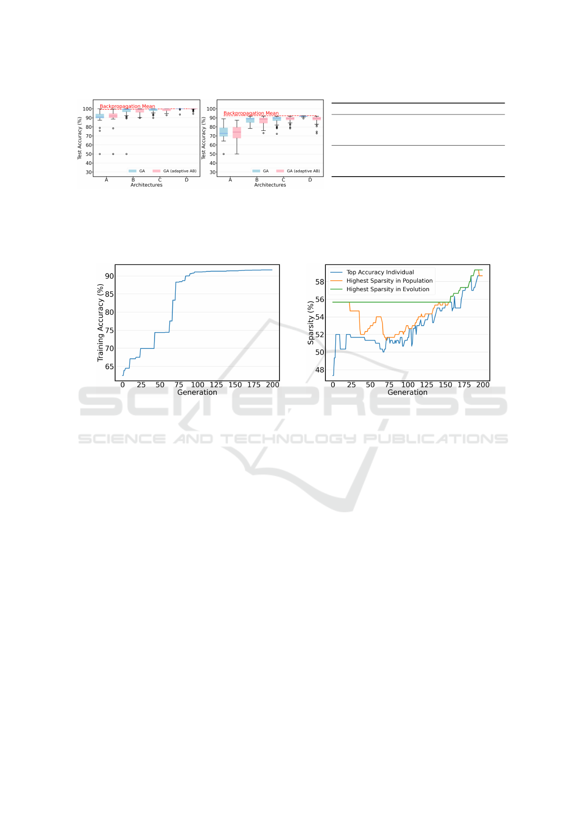
The results for the moons dataset are shown in

Fig. 3a. We observe that the GA is able to achieve

very high ﬁnal accuracies, reaching almost 100%

mean accuracy for network D. Examining the distri-

bution of the different GA runs for the various net-

work architectures, there exists a clear connection be-

tween the number of network parameters and the per-

formance. Whereas, for the smallest network A with

only 80 parameters, the mean difference to backprop-

agation is around 9%. The difference diminishes con-

tinuously with increasing parameter count. For net-

works C and D, the mean approximately matches that

of backpropagation, and for network D, there remains

only little variance between the runs. The difference

in performance between the different GA conﬁgura-

tions is less prominent. In general, the mean for the

runs using an accuracy bound is a little higher than

those that did not use it, but for increasing network

sizes, this effect plays less of a role.

The results on the circles dataset, illustrated in

Fig. 3b, mostly support these ﬁndings. Consider-

ing the mean performance of backpropagation, it be-

comes clear that the circles dataset has higher com-

plexity than the moons dataset. The GA, again, scores

the lowest accuracies on network architecture A but

reaches higher ﬁnal accuracies on the larger networks.

The highest mean accuracy of 91.6% is achieved on

network D, but this time without using an accuracy

bound. Also, there seems to be a certain minimum

threshold for the parameter count before which the ﬁ-

nal accuracies are noticeably lower, but increasing the

network size has less of an effect after exceeding it.

Still, we can say that there exist situations where the

GA is able to score very similar accuracies to back-

propagation.

To get an impression of the typical behavior of the

GA regarding the development of our accuracy and

sparsity objectives, we selected one high-performing

example run from the runs on the circles dataset;

that run was performed on network architecture B us-

ing the GA conﬁguration with an adaptive accuracy

bound. In Fig. 4a, we see that the individual with the

highest ﬁtness in the initial population had less than

65% accuracy. This accuracy is then successively im-

proved in the ﬁrst 100 generations, taking a set of

big leaps until the ﬁnal accuracy reaches a plateau

at around 91% accuracy. This clearly shows the op-

timization capabilities of the genetic algorithm. For

the next 100 generations, until the generation thresh-

old for GA (adaptive AB) is reached, only minor im-

provements are made. Meanwhile, Fig. 4b shows how

the sparsity develops over the course of the evolution.

Typical behavior is that the sparsity decreases in the

ﬁrst half of the generations since we prioritize achiev-

ing our accuracy goal, and only when the improve-

ment of the accuracy slows down does the optimiza-

tion of the sparsity really start to show. GA really

started to improve on the sparsity objective. That is

because, at that point, the population is very homoge-

neous, and there are many individuals with the same

accuracy. In this run, the GA achieved an additional

improvement of around 10% in sparsity compared to

the top individual in the initial population.

Scalability. Calculating the ﬁtness of the individu-

als in the population is the decisive factor on runtime

NCTA 2024 - 16th International Conference on Neural Computation Theory and Applications

454

(a) moons, R = 50 (b) circles, R = 50

Arch. GA GA (adaptive AB) Backprop.

moons

A 90.7% ± 7.2 90.9% ± 9.1 99.4% ± 2.4

B 96.9% ± 7.3 97.5% ± 3.3 99.6% ± 1.9

C 98.4% ± 2.5 98.9% ± 1.7 99.8% ± 1.4

D 99.8% ± 0.9 99.6% ± 1.0 99.9% ± 0.0

circles

A 73.9% ± 8.1 73.7% ± 8.6 92.3% ± 0.1

B 87.3% ± 3.6 86.8% ± 4.4 92.4% ± 0.0

C 88.0% ± 4.3 88.5% ± 3.2 92.3% ± 0.0

D 91.6% ± 0.5 88.3% ± 4.0 92.4% ± 0.0

Figure 3: Overview of the performance of the GA in the moons (a) and circles (b) datasets. The blue boxes contain different

runs for every architecture using the default GA conﬁguration. The pink boxes contain the results of R runs for the GA

conﬁguration that uses the adaptive accuracy bound with initial threshold value 0.85. For comparison, we added the mean

accuracies that were achieved with the trained networks using backpropagation. (c) summarizes the achieved accuracies.

(a) Accuracy (b) Sparsity

Figure 4: Optimization progress of one well-performing run using “GA (adaptive BA)” on network architecture B = [2,75, 2]

in the circles dataset with regard to the accuracy (a), and the sparsity (b). The blue line shows the sparsity of the ﬁttest

individual in the current population. The orange line displays the top sparsity in the current population, and the green line

represents the current best sparsity found in all previous generations.

complexity with O(g ∗ N ∗ (d ∗l ∗b

)) multiplications

for an evolution with g generations, a population of

size N, d dataset samples and a worst case network

architecture with l ∗ b

parameters (i.e., length of the

bit-vector). Typically N < g and (l ∗ b

) ≪ d. In prac-

tice, the effect of g ∗ N on the runtime can be reduced

by efﬁcient parallelization. A compressed version of

the subnetwork encoding reduces the complexity for

the other GA operations.

5.2 Edge-Popup & Weight Initialization

In the previous subsection, we saw that the GA per-

forms well on the given binary classiﬁcation tasks,

achieving accuracies that are very close to or even

match the accuracies obtained by training via back-

propagation, given a sufﬁcient network architecture

is chosen. To get an idea of how well the GA per-

forms in comparison to other methods that search

for SLTs in a randomly initialized neural network,

we repeat our previous experimental setup using the

well-known edge-popup algorithm (Ramanujan et al.,

2020). Edge-popup assigns a score to each weight

of the neural network and constructs subnetworks by

only choosing the top k% scoring edges in each layer

for the forward pass. The scores are updated in the

backward pass by using the straight-through gradi-

ent estimator (Bengio et al., 2013). Once pruned,

edges can re-appear in a subnetwork since the edges’

contribution to the loss is continuously re-evaluated

when approximating the gradients. The parameter

k in the forward pass denotes a ﬁxed value, which

is also called the pruning rate. Therefore, a prun-

ing rate of 60% corresponds to a subnetwork where

(1 − k) = 40% of weights are pruned. Note that the

sparsity metric we use in our work works the other

way around. A subnetwork with a sparsity of 60%

means 60% of weights are pruned.

We use the default settings from the authors and

train for a total of 100 epochs. Every conﬁguration

is evaluated on 25 random seeds. The authors found

two initialization methods that worked particularly

Finding Strong Lottery Ticket Networks with Genetic Algorithms

455

(a) moons, R = 25 (b) circles, R = 25

Figure 5: Illustration of the performance of edge-popup on shown datasets using the different color-coded initializations with

R runs each. The backpropagation mean accuracies on the respective architectures (dashed line) are provided for comparison.

well for their experiments: initializing the network

parameters from a Kaiming normal distribution (also

known as He initialization (He et al., 2015)), which

(following the notation of Ramanujan et al. (2020))

we refer to as “Weights ∼ N

”, or sampling from a

signed Kaiming constant distribution, which we refer

to as “Weights ∼ U

”. Thus, in addition to using our

initialization method, which we indicate as “Weights

∼ U

[−1,1]

”, we also consider runs where the networks

are initialized using both of their methods. Note that

we use the scaled versions of these methods, where

the standard deviation is scaled by

1/k. For the ex-

act deﬁnitions of these methods, refer to Ramanujan

et al. (2020). As with our GA, we also sample the

biases from the uniform distribution when using our

parameter initialization method with edge-popup.

Due to the considerable performance difference

between alternative parameter initializations for our

GA, which is also supported by the ﬁndings of Ra-

manujan et al. (2020), we start with an ablation study

to determine the highest accuracy achieving initial-

ization technique for edge-popup before proceeding

with the actual comparison studies. Fig. 5a shows

the results of the different runs edge-popup on the

moons dataset. The trend that the larger the network,

the higher the ﬁnal accuracies on the moons dataset

typically are, seems to apply here as well. It is also

noticeable that the runs using our parameter initial-

ization method (apart from network A) generally out-

performed the other run-throughs. In the case of net-

work D, it did so by quite a signiﬁcant margin (≈ 5%

mean difference). Nevertheless, in none of the set-

tings, edge-popup’s mean accuracy comes close to

the performance of backpropagation. The same holds

for the circles experiment, as shown in Fig. 5b, ex-

cept here, the Kaiming normal and signed Kaiming

constant distributions proved to be completely insuf-

ﬁcient. There is no run where the classiﬁcation accu-

racy is better than random, i.e., the predicted class la-

bel is correct in only 50% of cases. Considering these

results, one might assume that this is an algorithmic

issue, but since edge-popup performs well with our

initialization method, the issue has to be the Kaim-

ing normal or Kaiming singed constant distributions.

A potential reason might be the Gaussian nature of

the rings, which has a distorting effect on the meth-

ods. Finding the exact cause remains subject to future

work. In summary, it seems that at least for the moons

and circles datasets, edge-popup beneﬁts from us-

ing uniform initialization. Going forward, we, there-

fore, decided to sample the parameters for both the

GA and edge-popup from the same distribution.

Considering the contrary development of the ac-

curacy and sparsity levels at the beginning of the evo-

lution (cf. Fig. 4b), we hypothesize a correlation. This

also implies a potential connection between the num-

ber of pruned parameters throughout the evolution

and the ﬁnal achieved ﬁtness. Opposed to us, edge-

popup works with ﬁxed pruning rates. To rule out any

performance deﬁcits that might arise because of this

inﬂexibility, we include additional edge-popup runs in

our comparison study, where we set the pruning rates

to the mean sparsity levels that can be achieved with

the two GA conﬁgurations. We chose that conﬁgura-

tion for every architecture and dataset, which scored

the highest mean accuracy, and reran the edge-popup

experiments with the derived mean sparsity levels.

The results of our comparison study are depicted

in Fig. 6. For an extensive evaluation, we plotted the

mean accuracy of the best-performing GA conﬁgura-

tion for the respective architecture, together with the

mean accuracies of backpropagation and the original

edge-popup runs. The shaded area around the line

plots represents the 95% conﬁdence intervals for the

estimation of the mean. Relevant for the compari-

son of edge-popup with the adapted pruning rates, we

NCTA 2024 - 16th International Conference on Neural Computation Theory and Applications

456

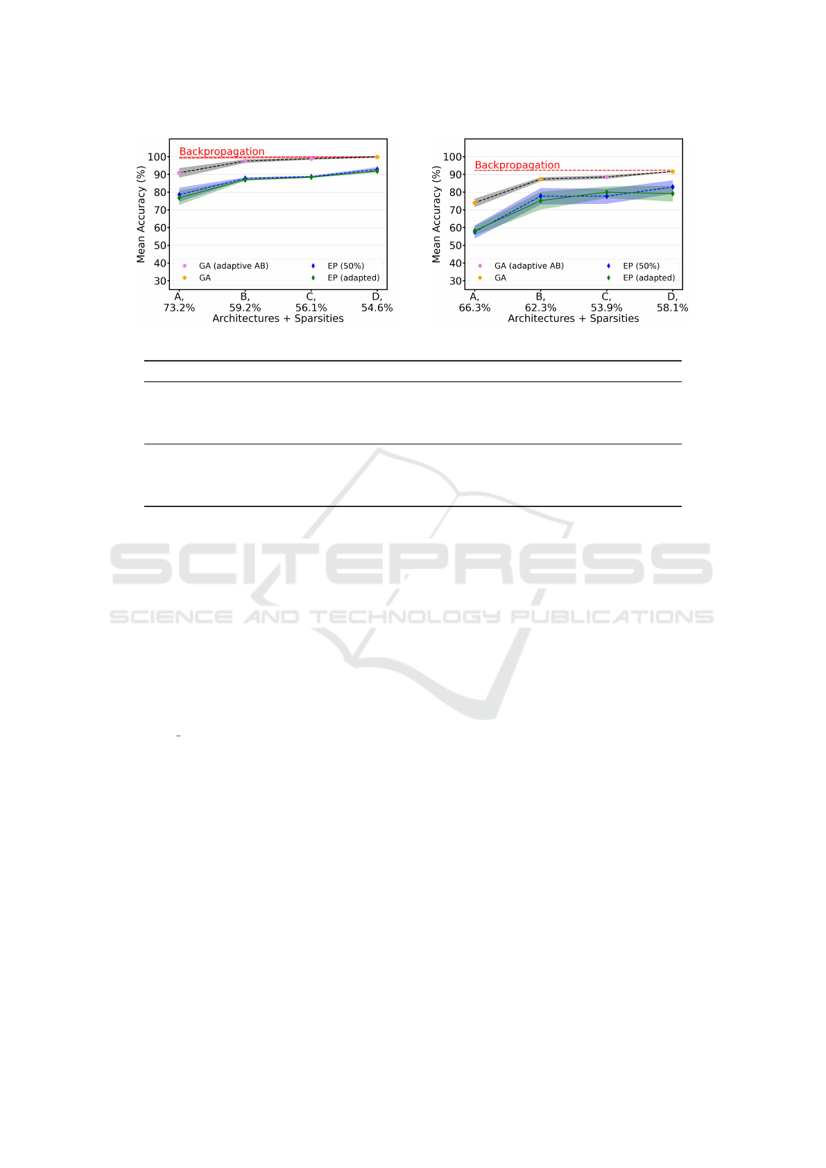
(a) moons (b) circles

Dataset Reference Target Coef. Std. Err. z P > |z| 95%-Conf.

moons

GA GA (adaptive AB) 0.042 0.083 0.507 0.612 [-0.121, 0.205]

EP (50%) EP (adapted) -0.133 0.095 -1.405 0.160 [-0.320, 0.053]

GA EP (50%) -1.185 0.081 -14.697 0.000 [-1.343, -1.027]

GA Backpropagation 0.661 0.087 7.609 0.000 [0.491, 0.831]

circles

GA GA (adaptive AB) -0.106 0.064 -1.670 0.095 [-0.231, 0.018]

EP (50%) EP (adapted) -0.062 0.102 -0.609 0.543 [-0.263, 0.138]

GA EP (50%) -0.964 0.074 -13.095 0.000 [-1.109, -0.820]

GA Backpropagation 1.030 0.071 14.595 0.000 [0.892, 1.168]

Figure 6: Performance evaluation of the GA against edge-popup on shown datasets, using the respective sparsity levels that

were achieved with our GA conﬁgurations as new values for the ﬁxed pruning rates. Depending on the achieved mean ac-

curacy, we either adapt the mean sparsity levels from “GA” or from “GA (adaptive AB)”, which is indicated by the different

colored dots. For comparison, we plot the mean accuracies and 95% conﬁdence intervals for the corresponding GA conﬁg-

uration, backpropagation, and the original edge-popup variant using the default prune-rate of 0.5. A ﬁnal statistical analysis

evaluates the performance difference of combinations of algorithms based on p-values for the GA and edge-popup conﬁgura-

tions, as well as the backpropagation baseline. (c) shows the performance deviation of the target algorithm from the reference.

speciﬁed the respective mean sparsity levels our GA

conﬁgurations achieved on the x-axis in addition to

the architectures. We can see in Fig. 6a that for moons,

these levels dropped with increasing network sizes,

converging to 0.5, which corresponds to edge-popup’s

default prune rate value. This suggests that the inﬂu-

ence of the varied pruning rate should be higher for

smaller architectures. Indeed, we observe the biggest

relative change for network A. The varied prune rate

appears to have a negative effect as it resulted in mul-

tiple low-accuracy runs, which negatively inﬂuenced

the mean. Yet, because of the high variance, there are

also some instances that scored higher compared to

EP (50%). For the other networks, there was little to

no change regarding the mean accuracy, and if there

was, it was only negative. The same holds true for

the circles dataset, as can be seen in Fig. 6b except

for architecture C. Since there is considerable vari-

ance between runs that use the same pruning rate and

the conﬁdence intervals mostly overlap, it cannot be

concluded with certainty that these changes are due to

the varied pruning rates. Overall, none of the changes

lead to a signiﬁcant performance improvement.

If we compare edge-popup against the GA con-

ﬁgurations, it becomes apparent that the GA outper-

forms for every dataset and architecture, even if we

enable edge-popup to ﬁnd sparser subnetworks. In

fact, the adapted pruning rates lead to a worse perfor-

mance. Based on this, we can conclude that the GA

can ﬁnd higher accuracy scoring subnetworks that are

also sparser and approximately match backpropaga-

tion for larger networks. To test the statistical signif-

icance of our ﬁndings, we ﬁt a linear mixed model to

our accuracy data. We are mainly interested in com-

paring the different algorithms across different archi-

tectures on the same dataset. That’s why we model the

algorithms as ﬁxed effects and treat the four architec-

tures and varying network initializations as random

effects to account for the variability across runs. We

perform our statistical analysis using the MixedLM

module from (Seabold and Perktold, 2010). To ﬁt

the data and ensure proper convergence, we employ

Powell’s algorithm, use the restricted maximum like-

lihood (REML), and standardize the accuracies. The

Finding Strong Lottery Ticket Networks with Genetic Algorithms

457

results of our analysis are listed in Table 6c.

For assessing the statistical signiﬁcance, we con-

sider various statistics, including coefﬁcients and p-

values, to determine the relationship between the ref-

erence algorithm and the target algorithm. Starting

with the moons dataset, we can see that the coefﬁcient

for GA (adaptive AB) is positive. This indicates that it

performs slightly better than the GA, considering all

architectures and initializations. Yet, because the p-

value is > 0.05, this performance difference is statis-

tically insigniﬁcant. The same holds for edge-popup

with the varied prune rate, although in this case, the

negative coefﬁcient indicates a slightly worse per-

formance of EP (adapted), supporting our previous

ﬁndings. Because both GA (adaptive AB) and EP

(adapted)’s performances deviate insigniﬁcantly from

the reference algorithms, we only compare GA and

EP (50%) against each other. Doing so, we observe

a large negative coefﬁcient, implying a considerably

worse performance of EP (50%). This result is sta-

tistically signiﬁcant, as the p-value is 0. Compared

to backpropagation, the GA conﬁguration performs

moderately worse, which is also a statistically sig-

niﬁcant result. For the circles dataset, the analysis

draws a very similar picture. Although, in this case,

GA (adaptive AB) has a negative coefﬁcient, support-

ing the (almost statically signiﬁcant) result that the

base GA conﬁguration is a more appropriate choice

for this dataset. Accounting for all random effects,

backpropagation here clearly outperforms the GA.

We conclude that the GA performs signiﬁcantly

better than edge-popup in the given scenarios and per-

forms only moderately worse than backpropagation

on the moons dataset regarding the ﬁnal accuracy.

5.3 Multi-Class Performance

So far, we only considered datasets for binary clas-

siﬁcation. It turns out that our approach has a much

harder time ﬁnding suitable lottery tickets for multi-

class classiﬁcation problems. We ﬁrst analyze that be-

havior by comparing the performance of the GA using

network architecture B

and the 2-, 3-, 4-, 5-, and 10-

class variants of the digits dataset.

The results are depicted in Fig. 7a. We observe

that, at least in the binary case, the GA still reaches

perfect accuracy in most of the runs; however, us-

ing just one more class label leads to a considerable

increase in variance. There are still runs that reach

approximately 100% accuracy, which is not the case

anymore for the 4-class and 5-class settings, where

Preliminary experiments showed the highest GA accu-

racies on this architecture in the computationally less inten-

sive base conﬁguration.

the variance further increases, and there is a notice-

able drop in achieved accuracy. When we reach the

10-class setting, the mean accuracy is only a little

above 54%. The increasing number of class labels

seems to pose a considerable challenge to the GA.

These observations also hold for much simpler

multi-class problems: For a follow-up experiment,

we introduce the blobs dataset consisting of up to

10 different 2-dimensional Gaussian-shaped clusters

with different class labels 1,...,10. These clusters are

uniformly distributed in the feature space and do not

overlap, as shown in Figure 7b. For this experiment,

we used a neural network architecture that consists of

2 input neurons, 100 hidden units, and as many output

neurons as required, given the number of classes. For

the classiﬁcation of points in 2d space, backpropaga-

tion is able to reach 100% accuracy regardless of the

number of classes. The results are shown in Fig. 7c

and draw a similar picture as the ﬁrst experiment:

While instances with fewer classes can reach perfect

accuracy, trying to distinguish more class labels leads

to increasingly bad ﬁnal accuracies. However, in con-

trast to the digits dataset, the GA can ﬁnd high-

accuracy subnetworks for a higher maximum number

of class labels (up to 6 classes), which suggests that

the GA can indeed deal with more classes when the

input space is less complex.

Aside from that, we observe a unique multi-modal

distribution of the accuracies, whose detailed analysis

is left for future work. At the moment, we reckon that

since the type of training we perform with our GA is

at its core just the task of solving a complex combi-

natorial problem, i.e., the problem of sampling proper

decision boundaries, the complexity of this task grows

superlinearly with an increasing number of decision

boundaries that need to be arranged in the feature

space. One observation we made during the GA runs

is that the accuracy is improved in only very small

steps, and the GA takes a long time to converge. This

behavior could partly be explained by the low popu-

lation diversity that leads to very homogenous popu-

lations already early in the evolution. In that phase,

the main driver of change is the mutation operation,

which can only lead to small accuracy improvements.

We hypothesize that it needs more sophisticated GA

operations, including proper diversity retention tech-

niques, to deal with complex multi-class datasets.

6 CONCLUSION

We have presented a GA-based approach for ﬁnd-

ing strong lottery ticket networks without any training

steps on the network. We have analyzed different con-

NCTA 2024 - 16th International Conference on Neural Computation Theory and Applications

458

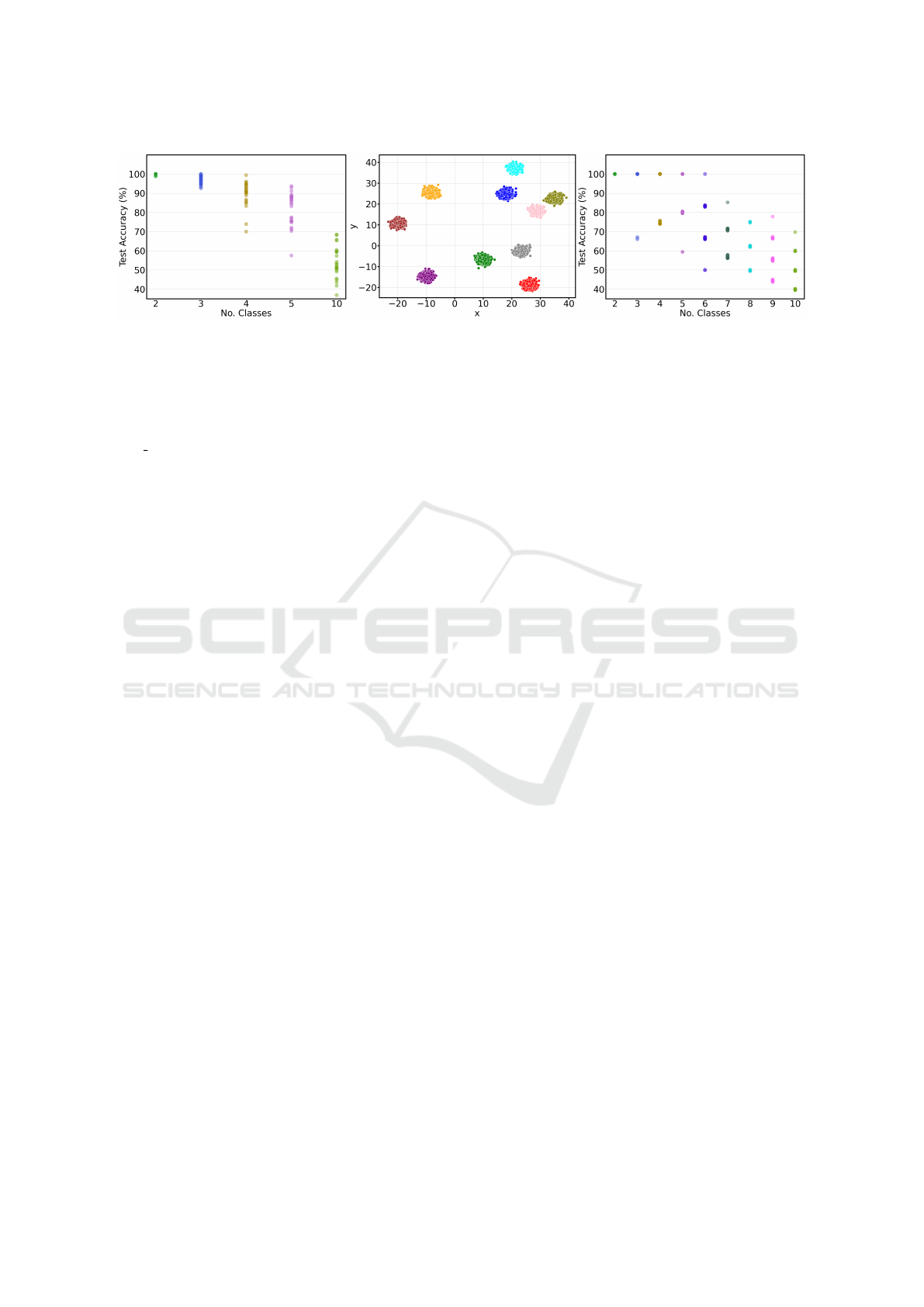
(a) digits, R=25 (b) blobs test dataset (c) blobs

Figure 7: Mutli-class performance on R runs: (a) Overview of the distribution of ﬁnal accuracies achieved by the GA (without

accuracy bound) for different variants of the digits dataset. For the binary case we consider class labels 0 and 1, for the

ternary case 0, 1, and 2, and so on. All runs were performed on architecture B (cf. Table 2c), but we adapted the number of

output neurons according to the number of class labels. (b) illustrates the blobs test dataset for 10 differently labeled cluster

of 2d points, generated using scikit-learn (Pedregosa et al., 2011). (c) Performance of default GA conﬁguration without

accuracy bound on the blobs dataset with varying class labels. The dataset was generated using the scikit-learn function

make blobs and consists of differently labeled clusters, each containing 1250 datapoints. For this experiment, we used a

network architecture [2,100, n] where n is the number of class labels.

ﬁgurations and behaviors of the GA and have shown

that, for simple binary classiﬁcation problems, our ap-

proach outperforms the start-of-the-art method edge-

popup by producing smaller and more accurate sub-

networks. This holds even when the latter is given a

more beneﬁcial weight initialization procedure. Fur-

thermore, we found that forcing edge-popup to pro-

duce subnetworks that possess the same sparsity lev-

els as the ones produced by the GA leads to a drop

in accuracy. Although integrating an adaptive accu-

racy bound resulted in slightly better accuracies on the

moons dataset, in our experiments, this effect is sta-

tistically insigniﬁcant and comes with reduced com-

putational efﬁciency, favoring the standard GA. Fi-

nally, we have also observed that the performance of

our approach breaks down when ﬁnding networks for

multi-class classiﬁcation problems. This poses sub-

stantial questions about the relationship between net-

work structure and learnability for future research.

Notably, in the shown example datasets, our GA-

based approach has the advantage over edge-popup,

which implements training steps via backpropagation

and thus depends on gradient information, which our

approach does not. This can be seen as a call to revisit

alternative methods of evolving neural networks, at

least for special cases. Since our approach effectively

frames the problem of ﬁnding a good neural network

as a problem of binary combinatorial optimization, it

may also open up new solving methods to this appli-

cation (see Whitaker (2022)) or allow for better inte-

gration of neural networks in scenarios where combi-

natorial optimization is already employed.

We would also like to point out that — since the

GA is not using gradient information — it is likely

that our approach has applications beyond classical

neural networks, which are built on functions that al-

low gradient information to pass through. We hypoth-

esize that using our GA, it should be possible to use

non-differentiable evaluation functions like the edit

distance (Levenshtein et al., 1966) for strings or logi-

cal consistency checks for propositional logic directly

as loss functions without requiring a potentially sub-

optimal differentiable surrogate (cf. Patel and Matas

(2021); Li and Srikumar (2019)) which would have

important implications for ﬁelds like natural language

processing or neural reasoning. To allow for the com-

parison to the state of the art, we chose classiﬁca-

tion problems for this paper; however, future work

should aim for more complex network structures that

allow for non-differentiable functions and test if our

approach — and thus a variant of the lottery ticket

hypothesis – still functions there.

ACKNOWLEDGEMENTS

This work was partially funded by the Bavarian Min-

istry for Economic Affairs, Regional Development

and Energy as part of a project to support the thematic

development of the Institute for Cognitive Systems.

REFERENCES

Aggarwal, C. C. et al. (2018). Neural networks and deep

learning. Springer, 10(978):3.

Bengio, Y., L

eonard, N., and Courville, A. (2013). Es-

timating or propagating gradients through stochastic

neurons for conditional computation. arXiv preprint

arXiv:1308.3432.

Finding Strong Lottery Ticket Networks with Genetic Algorithms

459

Chen, X., Zhang, J., and Wang, Z. (2021). Peek-a-boo:

What (more) is disguised in a randomly weighted neu-

ral network, and how to ﬁnd it efﬁciently. In Interna-

tional Conference on Learning Representations.

Frankle, J. and Carbin, M. (2018). The lottery ticket hypoth-

esis: Finding sparse, trainable neural networks. arXiv

preprint arXiv:1803.03635.

Gaier, A. and Ha, D. (2019). Weight agnostic neural net-

works. Advances in neural information processing

systems, 32.

He, K., Zhang, X., Ren, S., and Sun, J. (2015). Delv-

ing deep into rectiﬁers: Surpassing human-level per-

formance on imagenet classiﬁcation. In Proceedings

of the IEEE international conference on computer vi-

sion, pages 1026–1034.

Hinton, G., Vinyals, O., and Dean, J. (2015). Distilling

the knowledge in a neural network. arXiv preprint

arXiv:1503.02531.

Huang, G.-B., Zhu, Q.-Y., and Siew, C.-K. (2006). Extreme

learning machine: theory and applications. Neuro-

computing, 70(1-3):489–501.

Jackson, A., Schoots, N., Ahantab, A., Luck, M., and

Black, E. (2023). Finding sparse initialisations using

neuroevolutionary ticket search (nets). In Artiﬁcial

Life Conference Proceedings 35, volume 2023, page

110. MIT Press One Rogers Street, Cambridge, MA

02142-1209, USA journals-info . . . .

Kasun, L. L. C., Zhou, H., Huang, G.-B., and Vong, C. M.

(2013). Representational learning with elms for big

data. IEEE Intelligent Systems.

Lee, N., Ajanthan, T., and Torr, P. H. (2018). Snip: Single-

shot network pruning based on connection sensitivity.

arXiv preprint arXiv:1810.02340.

Levenshtein, V. I. et al. (1966). Binary codes capable of cor-

recting deletions, insertions, and reversals. In Soviet

physics doklady, volume 10, pages 707–710. Soviet

Union.

Li, T. and Srikumar, V. (2019). Augmenting neural net-

works with ﬁrst-order logic. In Proceedings of the

57th Annual Meeting of the Association for Compu-

tational Linguistics.

Malach, E., Yehudai, G., Shalev-Schwartz, S., and Shamir,

O. (2020). Proving the lottery ticket hypothesis: Prun-

ing is all you need. In International Conference on

Machine Learning, pages 6682–6691. PMLR.

Orseau, L., Hutter, M., and Rivasplata, O. (2020). Loga-

rithmic pruning is all you need. Advances in Neural

Information Processing Systems, 33:2925–2934.

Patel, Y. and Matas, J. (2021). Feds-ﬁltered edit distance

surrogate. In International Conference on Document

Analysis and Recognition, pages 171–186. Springer.

Pedregosa, F., Varoquaux, G., Gramfort, A., Michel, V.,

Thirion, B., Grisel, O., Blondel, M., Prettenhofer,

P., Weiss, R., Dubourg, V., et al. (2011). Scikit-

learn: Machine learning in python. Journal of ma-

chine learning research, 12(Oct):2825–2830.

Pensia, A., Rajput, S., Nagle, A., Vishwakarma, H., and

Papailiopoulos, D. (2020). Optimal lottery tickets via

subset sum: Logarithmic over-parameterization is suf-

ﬁcient. Advances in neural information processing

systems, 33:2599–2610.

Ramanujan, V., Wortsman, M., Kembhavi, A., Farhadi, A.,

and Rastegari, M. (2020). What’s hidden in a ran-

domly weighted neural network? In Proceedings

of the IEEE/CVF conference on computer vision and

pattern recognition, pages 11893–11902.

Seabold, S. and Perktold, J. (2010). statsmodels: Econo-

metric and statistical modeling with python. In 9th

Python in Science Conference.

Shevchenko, A. and Mondelli, M. (2020). Landscape con-

nectivity and dropout stability of sgd solutions for

over-parameterized neural networks. In International

Conference on Machine Learning, pages 8773–8784.

PMLR.

Tanaka, H., Kunin, D., Yamins, D. L., and Ganguli, S.

(2020). Pruning neural networks without any data by

iteratively conserving synaptic ﬂow. Advances in neu-

ral information processing systems, 33:6377–6389.

Wang, C., Zhang, G., and Grosse, R. (2020a). Picking

winning tickets before training by preserving gradient

ﬂow. arXiv preprint arXiv:2002.07376.

Wang, H., Qin, C., Bai, Y., Zhang, Y., and Fu, Y. (2021a).

Recent advances on neural network pruning at initial-

ization. arXiv preprint arXiv:2103.06460.

Wang, Y., Zhang, X., Xie, L., Zhou, J., Su, H., Zhang, B.,

and Hu, X. (2020b). Pruning from scratch. In Pro-

ceedings of the AAAI Conference on Artiﬁcial Intelli-

gence, volume 34, pages 12273–12280.

Wang, Z., Luo, T., Li, M., Zhou, J. T., Goh, R. S. M., and

Zhen, L. (2021b). Evolutionary multi-objective model

compression for deep neural networks. IEEE Compu-

tational Intelligence Magazine, 16(3):10–21.

Whitaker, T. (2022). Quantum neuron selection: ﬁnd-

ing high performing subnetworks with quantum al-

gorithms. In Proceedings of the Genetic and Evolu-

tionary Computation Conference Companion, pages

2258–2264.

Whitley, D., Tin

os, R., and Chicano, F. (2015). Optimal

neuron selection: Nk echo state networks for rein-

forcement learning. arXiv preprint arXiv:1505.01887.

Wortsman, M., Farhadi, A., and Rastegari, M. (2019). Dis-

covering neural wirings. Advances in Neural Informa-

tion Processing Systems, 32.

Wu, T., Li, X., Zhou, D., Li, N., and Shi, J. (2021).

Differential evolution based layer-wise weight prun-

ing for compressing deep neural networks. Sensors,

21(3):880.

Zhou, H., Lan, J., Liu, R., and Yosinski, J. (2019). De-

constructing lottery tickets: Zeros, signs, and the su-

permask. Advances in neural information processing

systems, 32.

NCTA 2024 - 16th International Conference on Neural Computation Theory and Applications

460