
Enhanced Missing Data Imputation Using Intuitionistic Fuzzy
Rough-Nearest Neighbor Approach
Shivani Singh
a
AN & SK School of Information Technology, Indian Institute of Technology Delhi, New Delhi, India
Keywords: Intuitionistic Fuzzy Rough Sets, k-Nearest Neighbourhood, Missing Data Imputation.
Abstract: The exponential growth of databases across various domains necessitates robust techniques for handling
missing data to maintain data integrity and analytical accuracy. Traditional approaches often struggle with
real-valued datasets due to inherent limitations in handling uncertainty and imprecision. Nearest
Neighbourhood algorithms have proven beneficial in missing data imputation, offering effective solutions to
address data gaps. In this paper, we propose a novel method for missing data imputation, termed Intuitionistic
Fuzzy Rough-Nearest Neighbourhood Imputation (IFR-NNI), which extends the application of intuitionistic
fuzzy rough sets to handle missing data scenarios. By integrating Intuitionistic Fuzzy Rough Sets into the
nearest neighbor imputation framework, we aim to overcome the limitations of traditional methods, including
information loss, challenges in managing uncertainty and vagueness, and instability in approximation
outcomes. The proposed method is implemented on real-valued datasets, and non-parametric statistical
analysis is performed to evaluate its performance. Our findings indicate that the IFR-NNI method
demonstrates excellent performance in general, showcasing its effectiveness in addressing missing data
scenarios and advancing the field of data imputation methodologies.
1 INTRODUCTION
The extraction of meaningful insights from data is
fundamental for understanding phenomena and
facilitating processes such as classification and
regression. Across diverse domains including science,
communication, and business, vast amounts of data are
generated and utilized. However, datasets frequently
encounter missing data due to various factors such as
input errors, faulty measurements, or non-responses in
assessments. For instance, in wireless sensor networks,
missing data is often inevitable due to sensor faults or
communication malfunctions (Li and Parker, 2014),
while in DNA microarray studies, missing data may
arise from insufficient resolution or image corruption
(Sun et al., 2010). Additionally, repositories like the
UCI Machine Learning Repository commonly contain
datasets with substantial proportions of missing values.
The presence of missing values poses significant
challenges, particularly in the context of machine
learning techniques, where interpretation and analysis
may be severely compromised. Consequently, missing
data imputation emerges as a critical issue across
a
https://orcid.org/0000-0001-7054-1193
scientific research communities, particularly in data
mining and machine learning domains (Aydilek and
Arslan, 2012; Nelwamondo et al., 2013).
Addressing missing values can be approached in
various ways. While simple strategies like deletion or
substitution with zero or mean values are common,
they often lead to information loss and bias in
assessments. Alternatively, imputation methods aim to
estimate missing values using statistical or machine
learning approaches. The nature of missing data can be
categorized into three types: missing completely at
random (MCAR), missing at random (MAR), and not
missing at random (NMAR) (Little and Rudin, 2019).
Understanding these categories is crucial for selecting
appropriate imputation techniques. Statistical methods
typically employ simple approaches like mean or mode
imputation, while machine learning-based methods
involve building models to predict missing values
(García-Laencina et al., 2010). Nearest Neighbour
(NN) based methods have gained popularity for
missing value imputation due to their accuracy and
simplicity. However, they require specifying the
number of neighbors and suffer from high time
Singh, S.
Enhanced Missing Data Imputation Using Intuitionistic Fuzzy Rough-Nearest Neighbor Approach.
DOI: 10.5220/0013015600003837
Paper published under CC license (CC BY-NC-ND 4.0)
In Proceedings of the 16th International Joint Conference on Computational Intelligence (IJCCI 2024), pages 399-407
ISBN: 978-989-758-721-4; ISSN: 2184-3236
Proceedings Copyright © 2024 by SCITEPRESS – Science and Technology Publications, Lda.
399

complexity and local optima issues. Conversely,
statistical methods may introduce bias and complexity,
relying on initial guesses and eigenvector
representations (Troyanskaya et al., 2001).
The use of rough set theory introduced by Pawlak
(2012) for missing data imputation is motivated by its
strength in handling vagueness and incompleteness in
data without requiring additional information. It
provides robust approximations and decision rules
directly from the dataset, ensuring both effectiveness
and interpretability. The use of intuitionistic rough
sets, rather than classical rough sets, further enhances
this capability by addressing both uncertainty and
vagueness through the inclusion of membership and
non-membership functions. This dual aspect offers a
more nuanced approximation, particularly useful in
scenarios with incomplete or imprecise data, where
classical rough sets may not fully capture the inherent
uncertainty.
In this paper, we introduce a novel approach to
missing data imputation, leveraging the combination
of Intuitionistic Fuzzy (IF) rough sets and the nearest
neighbour algorithm. By integrating IF rough sets
with NN estimation, we aim to capitalize on the
accuracy of NN methods while enhancing noise
tolerance and robustness. Specifically, we propose IF
rough-nearest neighbour imputation methods. The
subsequent sections of this paper are organized as
follows: Section 2 reviews relevant literature. Section
3 provides essential preliminaries to understand the
theoretical background. Section 4 introduces the
proposed methodologies. Section 5 presents the
implementation of these methods on benchmark
datasets and evaluates their performance using non-
parametric statistical analysis. Finally, Section 6
concludes our work and outlines future research
directions.
2 LITERATURE REVIEW
Various domains such as meteorology,
transportation, and others have witnessed the
treatment of missing-valued data by researchers.
Although several algorithms with different
approaches have been proposed, they are not
commonly employed for specific domains or datasets.
Notable imputation techniques frequently used across
fields include those based on Nearest Neighbours
(NN), which predict missing values based on
neighboring instances. While NN methods offer
accuracy and simplicity, they come with drawbacks
such as the need for specifying the number of
neighbors, high time complexity, and local optima
issues.
Troyanskaya et al. (2001) proposed two methods,
KNN and SVD, for imputation in DNA microarrays.
KNN computes a weighted average of values based
on Euclidean distance from the K closest genes, while
SVD employs an expectation maximization (EM)
algorithm to approximate missing values. Comparing
the two, KNN showed greater robustness, particularly
with increasing percentages of missing values. Batista
and Monard (2003) introduced the k-nearest neighbor
imputation (KNNI) method, which replaces missing
values with the mean value of specific attribute
neighbors. Grzymala-Busse (2005) introduced global
most common (GMC), global most common average
(GMCA) methods for nominal and numeric
attributes, respectively, where missing values are
replaced by the most common or average attribute
values. Kim et al. (2005) proposed the local least
squares imputation (LLSI) method, which estimate
missing attribute values as a linear combination of
similar genes selected through k-nearest neighbors.
Schneider (2001) introduced an algorithm based
on regularized Expectation-Maximization (EM) for
missing value prediction, utilizing Gaussian
distribution to parameterize data and iteratively
maximizing likelihoods. Oba et al. (2003) proposed
Bayesian PCA imputation (BPCAI), incorporating
Bayesian estimation into the approximation stage.
Honghai et al. (2005) presented SVM-based
imputation methods, utilizing Support Vector
Machines and Support Vector Regressors.
Clustering-based methods, such as those by Li et al.
(2004) and Liao et al. (2009), use techniques like K-
means and Fuzzy k- means for imputation, often
incorporating sliding window mechanisms for data
stream handling. Neural network-based methods,
including Multi-Layer Perceptrons (MLP) (Sharpe
and Sholly, 1995), Recurrent Neural Networks
(RNN) (Bengio and Gingras, 1995), and Auto
Associative Neural Networks (AANN) (Pyle, 1999),
have been employed for imputation, each with its own
approach and advantages. Amiri and Jensen (2016)
introduced fuzzy rough set-based nearest neighbor
algorithms for imputation, showing superior
performance compared to traditional methods. In the
paper (Pereira et al., 2020), the adaptability of
Autoencoders in handling various types of missing
data are discussed.
While clustering-based algorithms often exhibit
high computational complexity, those based on
nearest neighbors are preferred for their
computational efficiency. Intuitionistic Fuzzy (IF) set
theory, known for effectively handling vagueness and
FCTA 2024 - 16th International Conference on Fuzzy Computation Theory and Applications
400

uncertainty, remains unexplored in missing value
imputation. In this work, we propose a missing data
imputation method based on IF rough-nearest
neighbor approach.
3 PRELIMINARIES
In this section a basic overview on Intuitionistic fuzzy
rough sets (IFRS) is given.
Definition 3.1. (Huang, 2013): A quadruple IS = (U,
AT, V, h) is called an Information System, where U
= {u
1
,u
2
,...,u
n
} is a non-empty finite set of objects,
called the universe of discourse, AT = {a
1
, a
2
,…, a
m
}
is a non-empty finite set of attributes.
where Va is the set of attribute values associated with
each attribute aAT and h:U×AT→V is an
information function that assigns particular values to
the objects against attribute set such that a AT, u
U and h(u, a) Va.
An information system IS = (U, AT, V, h) is said
to be a Decision System if AT = C D where C is a
non-empty finite set of conditional features/attributes
and D is a non-empty collection of decision
features/attributes with C ∩ D = . Here V = V
C
∪ V
D
V
D
with V
C
and V
D
as the set of conditional attribute
values and decision attribute values, respectively.
Definition 3.2. (Pawlak, 2012): Let IS = (U, AT, V,
h) be a decision system. For P AT, a P-
indiscernibility relation is defined as:
where, RP is an equivalence relation and [x]RP
divides the set U into equivalence classes defined by
the attributes belongs to P. If A U, then the lower
and upper approximation of set A are given by:
All the data instances that contained in set
must contained in set A while the instances that
contained in
may be a member of A.
Definition 3.3. (Atanassov, 1999): Given a non-
empty finite universe of discourse U. A set A on U
having the form A = {x, μ
A
(x),ν
A
(x)|x U} is
said to be an IF set, where μ
A
: U → [0, 1] and ν
A
:
U → [0, 1] with the condition 0 ≤ μ
A
(x) + ν
A
(x) ≤
1,x U are known as membership degree and non-
membership degree of the element x in A,
respectively. π
A
(x) = 1 − μ
A
(x) − ν
A
(x) is the
degree of hesitancy of the element x in IF set A.
The cardinality of an IF set A is given by
where 1 in numerator is a
translation factor that guarantees the positivity of |A|
while 2 in denominator is a scaling factor which
bounds the cardinality between 0 and 1.
An ordered pair μ, ν is called an IF value, where
0≤μ+ν≤1 and 0 ≤μ ,ν≤1. An information system is
said to be an IF information system if attribute values
corresponding to objects are IF value.
Properties: For every two IF Sets A and B the
following relations and operations hold:
2.
3.
4.
5.
, and
otherwise.
6.
7.
where, N is a negation operator.
Definition 3.4. (Bustince and Burillo, 1996): An IF
binary relation R(x
i
,x
j
) = μ
A
(x
i
, x
j
), ν
A
(x
i
, x
j
)
between objects x
i
, x
j
∈ U is said to be an IF
tolerance relation if it is reflexive (i.e., μ
A
(x
i
, x
i
) =
1 and ν
A
(x
i
, x
i
) = 0,∀x
i
∈ X) and symmetric (i.e.,
μ
A
(x
i
, x
j
) = μ
A
(x
j,
, x
i
) and ν
A
(x
i
, x
j
) = ν
A
(x
j
,
x
i
),∀x
i
, x
j
∈ X).
Let U be a collection of finite objects and C ⊆A,
an IF tolerance relation R
c
(x
i
,x
j
) =
μ
R
c
(x
i
,x
j
),ν
R
c
(x
i
,x
j
), c ∈ C is defined as:
(1)
Enhanced Missing Data Imputation Using Intuitionistic Fuzzy Rough-Nearest Neighbor Approach
401

Definition 3.5. (Cornelis et al., 2003): An IF
triangular norm or IF t-norm T is a mapping from [0,
1] × [0, 1] → [0, 1] which is increasing, associative
and commutative and satisfies T(1,x) = x, x [0,1].
An IF implicator I is a mapping [0, 1] × [0, 1] →
[0, 1], which is decreasing in its first component and
increasing in second component with condition I (0,
0) = 1 and I (1, x) = x, x [0, 1].
Example 3.1: If x = x
1
,x
2
and y = y
1
,y
2
in [0, 1]
are two IF values then an IF t-norm and IF implicator
are given as:
(2)
(3)
Definition 3.6. (Cornelis et al., 2003): Given an IF set
X U and R(x
i
,x
j
) is an IF similarity/tolerance
relation from U×U → [0,1] which assigns degree of
similarity to each distinct pair of objects. The lower
and upper approximation of X by R can be computed
in many ways. A general definition is given as:
(4)
(5)
Here, I is an IF implicator and T is an IF t-norm and
X(x
j
) = 1, for x
j
X, otherwise X(x
j
) = 0. The pair
,
is called as IF rough set.
4 PROPOSED METHODOLOGY
Jensen and Cornelis introduced the model based on
KNN algorithm using fuzzy-rough lower ap-
proximation and upper approximation in which
discrete or continuous decision attribute values of
datasets are predicted (Jensen and Cornelis, 2011).
Based on this methodology Amiri and Jensen
extended the FRNN model to predict the missing
values presented in the dataset (Amiri and Jensen,
2016). We have further extended this KNN based
algorithm for IF information system to impute the
missing values in IF information system using IF
rough sets approach.
In this subsection, IF rough approximation
operators are defined to achieve the target of missing
value imputation. This algorithm proposes that for
each instance/object of the dataset consisting at least
one missing value, that instance will be treated as
decision attribute and based on that attribute
prediction is made. We address this algorithm as IF
rough nearest neighbour imputation (IFRNNI).
4.1 If Rough Approximation Operators
Definition 4.1: The IF distance matrix d(y, z) for the
difference between instances y U and z U in order
to calculate the distance between the instances y =
μ
1
,ν
1
and z = μ
n
,ν
n
is defined as (Szmidt and
Kacprzyk, 2001):
(6)
where
Definition 4.2: IF similarity values for R(y, z), R
a
(y,
z), R
c
(y, z) and R
d
(y, z) with attribute a, conditional
attributes c’s and decision attribute d are defined as:
R(y, z) = min R
a
(y, z) = min (R
c
(y, z), R
d
(y, z)) (7)
where
Definition 4.3: The lower approximation and upper
approximation of instance y with respect to z are
defined as in the following equations:
R ↓ R
d
z(y) =
I(R(y, p), R
c
(p, z)) (8)
R ↑ R
d
z(y) =
T(R(y, p), R
c
(p, z)) (9)
where, N is the k-nearest neighbour of instance y. R
d
z
is an IF tolerance relation which determines the
similarities of two objects for the decision attribute.
R
d
(p,z) is also an IF tolerance relation which
measures the similarity of objects z and p with respect
to decision attribute d. In general, R
a
z(p) signifies the
similarity of objects z and p with respect to attribute
a. Here, all IF tolerance relations are computed by Eq.
(1).
One of the problems that are worth considering is
in the process of computing the distance between two
objects consisting of some missing attributes. Here,
we simply avoid missing attributes while computing
distances. Hence, the distance is only calculated
between those instances having non- missing attribute
values.
4.2 Prediction of Missing Values
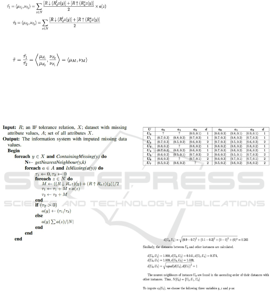
Definition 4.6. With the help of lower and upper
approximation operators,
and
are defined as
FCTA 2024 - 16th International Conference on Fuzzy Computation Theory and Applications
402
follows:
(10)
Definition 4.7. The predicted missing value, namely
, obtained with the help of
and
is defined as:
(11)
It is quite possible sometimes, that either
or
.
In such case,
/
cannot be estimated. To handle
this situation, the mean value of the attribute for the
neighbours is employed.
4.3 Algorithm and Illustrative Example
Algorithm 1: Missing Data Imputation using IFRNNI.
The above algorithm work as follows: In a dataset
domain, for every instance y, comprising at least one
missing data value for attribute a, the algorithm
obtains its k nearest neighbours and places them in
the set N. Partial similarities between units are
computed by considering the subset of all attributes
not missed for the two considered units. For instance,
in Example 4.1, the similarity between
and
is
determined using attributes
and ; between
and
, the attributes
,
, and are used; and
between
and
, only the decision attribute is
used due to missing values in other attributes. This
approach ensures that the similarity measure is as
comprehensive as possible based on the available
data. Thereafter, the missing value are approximated
utilizing y
'
s nearest neighbours. Next step is to
compute the lower approximation and upper
approximation of y with respect to the instance z,
utilizing the average of these, obtain the final
membership
and non-membership
of the
predicted value. The process is conducted for all the
instances which belong to N, and depending upon
these calculations over all the neighbours, the
algorithm returns a value.
Example 4.1: Two datasets are shown in Table 1. The
right side of the Table represents the original data
with no missing values while the left side represents
the same data with some missing attribute values
inserted. Missing values are epitomized by “?”. The
method of evaluating missing values by IF nearest
neighbour algorithm is as follows.
Table 1: Incomplete intuitionistic fuzzy value dataset.
In this IF decision system instance U
0
has two
missing values a
0
and a
1
, respectively. First, we
choose attribute value a
0
(U
0
) for imputation.
We calculate Euclidean distance between U
0
and
other instances given by Eq. (6). Since attribute value
a
1
(U
0
) is also missing, so we ignore this attribute at
the time of calculating distances and we get the
distance between U
0
and U
1
as;
y = U
0
is the instance having missing attribute value
c
0
(U
0
) and z, p N(y). We first take z = U
3
. On
putting third variable p = z in the formulae of
approximation operators, we get no new information.
So, we ignore this state and choose value of p other
than z, either U
1
or U
4
. We calculate the IF tolerance
relations by Eq. (1) and all the missing attribute
values are ignored in the calculation
Enhanced Missing Data Imputation Using Intuitionistic Fuzzy Rough-Nearest Neighbor Approach
403
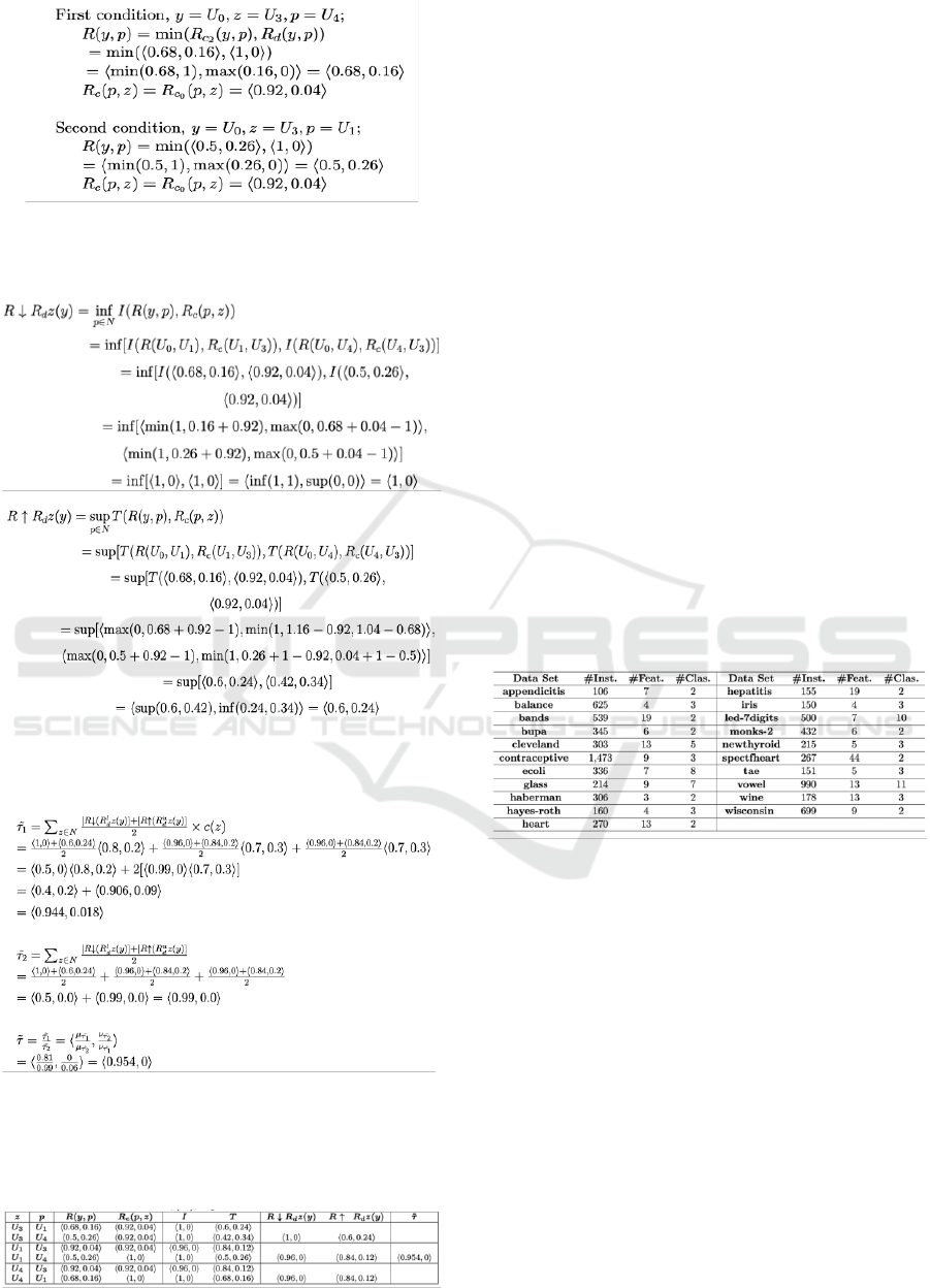
Now, putting the above values in the lower and
upper approximation given by Eq.(10), we get
Table 2 illustrates the computation of lower and
upper approximations using IF T-norm and IF
Implication across various attribute pairs.
Thus, we get the final predicted value of a
0
(U
0
) =
0.954, 0.
Table 2: a
0
(U
0
) imputation with IFRNNI.
5 EXPERIMENTAL ANALYSIS
In this section, some experiments are performed on
real valued dataset implementing the proposed
models and comparison is made with other existing
imputation techniques. The impact on the proposed
models with variation of parameter k for its different
values is investigated. A non- parametric statistical
test is also performed for the validation of the results.
5.1 Experimental Setup
This subsection describes the datasets used, the other
imputation methods used for comparison and also the
criteria employed for the comparison. An effective
way of estimating imputation methods is that first
values are artificially removed from the datasets and
then comparison is made between the imputed values
produced by the proposed method and the original
data values. For this purpose, we have employed 21
datasets from the KEEL dataset repository (Derrac et
al., 2015). Table 3 presents the short details of the
datasets utilized in the experimentation section. Since
none of the datasets include the missing data values,
we insert random missing values into them.
Table 3: Description of dataset.
Here, MCAR method is used for insertion of
missing values in the datasets. For the investigation
of the execution of the algorithms under various
conditions, we eliminate 5%, 10%, 20% and 30% of
the values in the datasets. Perhaps, anything above 30
percent could be too damaging to the data to obtain
useful results. A measure is required to compare the
results obtained from the imputation algorithms. A
commonly used measure to get the difference
between the values predicted by a model and the
values actually observed in the environment at which
experiment is performed, is the Root Mean Square
Error (RMSE) (also referred to as root mean square
deviation, RMSD). The RMSE of a model being used
for prediction with respect to the estimated variable
z
model
is defined as:
FCTA 2024 - 16th International Conference on Fuzzy Computation Theory and Applications
404
where, z
obs
is the observed value and z
model
is the
imputed value. RMSE measure is used here to
compare the yields of the imputation algorithms.
Since this measure generates values in different
ranges depending upon the ranges of attributes of
datasets, we have normalized the employed data with
the min-max normalization procedure (Shalabi et al.,
2006) so that the comparisons of RMSE values are
more practical.
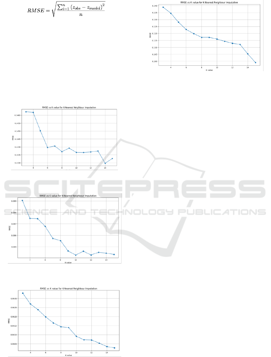
5.2 Effect of Parameter K
Figure 1: Average RMSE acquired by the algorithm with
5% missing values.
Figure 2: Average RMSE acquired by the algorithm with
5% missing values.
Figure 3: Average RMSE acquired by the algorithm with
5% missing values.
Figure 4: Average RMSE acquired by the algorithm with
5% missing values.
We first begin the experimentation in search
algorithms. These parameters are the distance
measures, similarity measures, IF t-norms, IF
implicators, IF quantifiers, OWA operators and
number of neighbours in which most of the best
values have been ascertained by other researchers. All
these parameters have previously been suggested in
section 4. For all other methods the parameters are
chosen based on suggestions in (Amiri and Jensen,
2016). The only parameter that needs to be laid down
is the number of neighbours, k. To observe the effect
of this parameter, we use 21 datasets together with
5%, 10%, 20% and 30% missing values injected into
the dataset. The tested values of the parameter k are
taken in the range 3 to 15. For the overall
convenience, only the average results are given here
which are shown in Figures 1-4.
5.3 Comparison with Other Missing
Data Imputation Methods
In this subsection, a comparison is made between the
proposed methods and the other imputation methods.
We have compared the proposed methods on 21
datasets with 14 missing value imputation methods
using different approaches that are described in
introduction section; namely, BPCAI, CMCI, FKMI,
KMI, KNNI, LLSI, MCI, SVDI, SVMI and WKNNI,
EMI, FRNNI, VQNNI and OWA-FRNNI (Amiri and
Jensen, 2016). The average RMSE results of all
methods are shown in Figure 5. It can be observed
from the figures that for all 5%, 10%, 20% and 30%
missing values that the proposed IFRNNI method,
have minimum average RMSE values as compared to
other imputation methods.
K-value
Enhanced Missing Data Imputation Using Intuitionistic Fuzzy Rough-Nearest Neighbor Approach
405
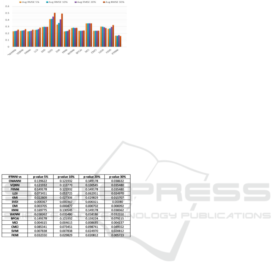
Figure 5: Average RMSE obtained from Missing Data
Imputation Algorithms.
Table 4 depicts the obtained results for IFRNNI
vs other imputation methods, and it shows that when
5%,10% and 20% values are missing from the
datasets, IFRNNI method has outperformed than
most of the imputation methods except FRNNI,
VQNNI, OWA-FRNNI, KNNI, BPCAI. The reason
is that obtained asymptotic p-values are less than the
0.05 level of significance. For 30% missing data
values, IFRNNI has outperformed all other
imputation methods.
Table 4: Comparison of the imputation algorithms with
IFRNNI in terms of RMSE.
6 CONCLUSION
Our study introduces novel methods for missing data
imputation by integrating IF rough set theory to
nearest neighbour approach. This fusion of
frameworks offers a comprehensive approach to
addressing missing values, leveraging Rough Set
Theory’s ability to handle uncertainty and IF set
theory’s representation of vagueness. Through
empirical evaluations on benchmark datasets, our
proposed methods demonstrate superior accuracy and
robustness compared to traditional techniques.
Notably, our methods offer simplicity and ease of
implementation, enhancing their practicality for real-
world applications. Overall, this research contributes
to advancing missing data imputation methodologies
and opens new avenues for leveraging theoretical
foundations to improve data analysis techniques
across various domains.
In future work, we will compare the
computational efficiency, ease of implementation,
interpretability, and generalization capabilities of
IFR-NNI with neural network-based imputation
methods, focusing on their performance across
diverse datasets.
REFERENCES
Li, Y., Parker, L. E. (2014). Nearest neighbor imputation
using spatial–temporal correlations in wireless sensor
networks. Information Fusion, 15, 64-79.
Sun, Y., Braga-Neto, U., Dougherty, E. R. (2010). Impact
of missing value imputation on classification for DNA
microarray gene expression data—a model-based
study. EURASIP Journal on Bioinformatics and
Systems Biology, 1-17.
Aydilek, I. B., Arslan, A. (2012). A novel hybrid approach
to estimating missing values in databases using k-
nearest neighbors and neural networks. International
Journal of Innovative Computing, Information and
Control, 7(8), 4705-4717.
Nelwamondo, F. V., Golding, D., Marwala, T. (2013). A
dynamic programming approach to missing data
estimation using neural networks. Information
Sciences, 237, 49-58.
Little, R. J., Rubin, D. B. (2019). Statistical analysis with
missing data (Vol. 793). John Wiley & Sons.
García-Laencina, P. J., Sancho-Gómez, J. L., Figueiras-
Vidal, A. R. (2010). Pattern classification with missing
data: a review. Neural Computing and
Applications, 19, 263-282.
Troyanskaya, O., Cantor, M., Sherlock, G., Brown, P.,
Hastie, T., Tibshirani, R., ..., Altman, R. B. (2001).
Missing value estimation methods for DNA
microarrays. Bioinformatics, 17(6), 520-525.
Batista, G. E., Monard, M. C. (2003). An analysis of four
missing data treatment methods for supervised
learning. Applied artificial intelligence, 17(5-6), 519-
533.
Grzymala-Busse, J. W., Grzymala-Busse, W. J. (2005).
Handling Missing Attribute Values. Data Mining and
Knowledge Discovery Handbook, 37.
Kim, H., Golub, G. H., Park, H. (2005). Missing value
estimation for DNA microarray gene expression data:
local least squares imputation. Bioinformatics, 21(2),
187-198.
Schneider, T. (2001). Analysis of incomplete climate data:
Estimation of mean values and covariance matrices and
imputation of missing values. Journal of climate, 14(5),
853-871.
Oba, S., Sato, M. A., Takemasa, I., Monden, M.,
Matsubara, K. I., Ishii, S. (2003). A Bayesian missing
value estimation method for gene expression profile
data. Bioinformatics, 19(16), 2088-2096.
FCTA 2024 - 16th International Conference on Fuzzy Computation Theory and Applications
406

Honghai, F., Guoshun, C., Cheng, Y., Bingru, Y., Yumei,
C. (2005). A SVM regression-based approach to filling
in missing values. In International Conference on
Knowledge-Based and Intelligent Information and
Engineering Systems (pp. 581-587). Berlin, Heidelberg:
Springer Berlin Heidelberg.
Li, D., Deogun, J., Spaulding, W., Shuart, B. (2004).
Towards missing data imputation: a study of fuzzy k-
means clustering method. In Rough Sets and Current
Trends in Computing: 4th International Conference,
RSCTC 2004, Uppsala, Sweden, June 1-5, 2004.
Proceedings 4 (pp. 573-579). Springer Berlin
Heidelberg.
Liao, Z., Lu, X., Yang, T., Wang, H. (2009). Missing data
imputation: a fuzzy K-means clustering algorithm over
sliding window. In 2009 Sixth International
Conference on Fuzzy Systems and Knowledge
Discovery (Vol. 3, pp. 133-137). IEEE.
Sharpe, P. K., Solly, R. J. (1995). Dealing with missing
values in neural network-based diagnostic systems.
Neural Computing & Applications, 3, 73-77.
Bengio, Y., Gingras, F. (1995). Recurrent neural networks
for missing or asynchronous data. Advances in neural
information processing systems, 8.
Pyle, D. (1999). Data preparation for data mining. Morgan
Kaufmann.
Amiri, M., Jensen, R. (2016). Missing data imputation
using fuzzy-rough methods. Neurocomputing, 205,
152-164.
Pereira, R. C., Santos, M. S., Rodrigues, P. P., Abreu, P. H.
(2020). Reviewing autoencoders for missing data
imputation: Technical trends, applications and
outcomes. Journal of Artificial Intelligence
Research, 69, 1255-1285.
Huang, S. Y. (Ed.). (2013). Intelligent decision support:
handbook of applications and advances of the rough
sets theory.
Pawlak, Z. (2012). Rough sets: Theoretical aspects of
reasoning about data (Vol. 9). Springer Science &
Business Media.
Atanassov, K. T. (1999). Intuitionistic fuzzy sets (pp. 1-
137). Physica-Verlag HD.
Bustince, H., Burillo, P. (1996). Vague sets are
intuitionistic fuzzy sets. Fuzzy sets and systems, 79(3),
403-405.
Cornelis, C., De Cock, M., Kerre, E. E. (2003).
Intuitionistic fuzzy rough sets: at the crossroads of
imperfect knowledge. Expert systems, 20(5), 260-270.
Jensen, R., & Cornelis, C. (2011). Fuzzy-rough nearest
neighbour classification. In Transactions on rough sets
XIII(pp. 56-72). Springer Berlin Heidelberg.
Szmidt, E., & Kacprzyk, J. (2001). Entropy for intuitionistic
fuzzy sets. Fuzzy sets and systems, 118(3), 467-477.
Derrac, J., Garcia, S., Sanchez, L., Herrera, F. (2015). Keel
data-mining software tool: Data set repository,
integration of algorithms and experimental analysis
framework. J. Mult. Valued Logic Soft Comput, 17,
255-287.
Al Shalabi, L., Shaaban, Z., Kasasbeh, B. (2006). Data
mining: A preprocessing engine. Journal of Computer
Science, 2(9), 735-739.
Enhanced Missing Data Imputation Using Intuitionistic Fuzzy Rough-Nearest Neighbor Approach
407
