Modelling and Analysis of Spread Characteristics of Arbovirus Infections
Paolo Di Giamberardino
a
and Daniela Iacoviello
b
Department of Computer, Control and Management Engineering Antonio Ruberti, Sapienza University of Rome, Italy
Keywords:
Compartmental Model, Qualitative Model Analysis, Model Identification, Dengue Disease.
Abstract:
The problem of the definition of a mathematical model for epidemics, where the virus transmission is op-
erated by an infected vector like an insect, is addressed. Through the consideration of a small number of
compartments, in order to keep the mathematical analysis affordable, a five dimensional model is proposed
and, successively, used for the analysis of the main characteristics of the disease. Closed form expression are
then obtained for the equilibria, the stabiliy conditions and the reproduction number. Some numerical results
referring to the dengue disease emergency are also presented, firstly to identify the unknown model parameters
and then to validate the effectiveness of the model itself. Using such a model, some considerations on the most
effective action lines for spidemic containment are discussed.
1 INTRODUCTION
Globalization and climate change make the problem
of epidemics spread an emergency to be addressed
with coordinated strategies, acting promptly with pre-
ventive campaigns, firstly for geographical contain-
ment, and then for possible eradication.
An effective approach to the problem makes use
of mathematical models for description, analysis, pre-
diction and control the diseases evolution (Di Gi-
amberardino et al., 2019; Attaullah and Sohaib, 2020;
Di Giamberardino et al., 2021; Diagne et al., 2021;
Ayele et al., 2021; Di Giamberardino and Iacoviello,
2021; Alutto et al., 2024). In particular, arboviruses
are diseases (zoonoses) caused by agents (viruses)
transmitted from animals (arthropod vectors) to hu-
mans, through bites or stings. Among the arboviruses,
dengue, yellow fever, chikungunya and Zika viruses
are currently an emergency in tropical and sub-
tropical areas, involving almost 4 billion of people;
due to this growing threat, the World Health Organi-
zation (WHO) launched the Global Arbovirus Initia-
tive on March 31, 2022, proposing a plan to tackle
arboviruses threat by means of pandemic prevention,
risk analysis, communication and coordination.
For the particular case of the dengue, there has
been an increment in the last years, from 505430
cases in 2000 to more than 5 million in 2019, with
a spike of 6.5 million cases in 2023 and with about
a
https://orcid.org/0000-0002-9113-8608
b
https://orcid.org/0000-0003-3506-1455
7300 deaths reported. It is estimated that up to
400 million infections are occurring in the last years,
putting approximately half of the world’s population
at risk, (CDC, 2024). This viral infection is trans-
mitted to humans by the bite of infected mosquitoes,
mainly the Aedes aegypti one; the mosquitoes can
get the virus when they bite a subject in a symp-
tomatic, presymptomatic or asymptomatic condition,
especially when the patients have high fever or with
significant viremia.
Generally, individuals infected by dengue do not
have symptoms, loosing the viral load after 2 weeks.
Symptoms can appear about 1 week after the infec-
tion and last at most for a week; they include fever,
headache, nausea, rash; severe symptoms include ab-
dominal pain, persistent vomiting with blood, feeling
weak also for several weeks. Severe dengue generally
occurs with a second infection; the mortality among
severely infected individuals is quite high, with even
20% of fatalities.
Up to now, there is no specific treatment for severe
dengue and the current therapy generally focuses on
treating pain symptoms; the early detection with ac-
cess to medical care can reduce fatality rates (WHO,
2024a).
The first containment measure is prevention, act-
ing to reduce the possibility of mosquitoes bites: win-
dow screens, mosquitoes repellents and use of clothes
covering as much of the body as possible. Moreover,
mosquito breeding can be prevented by suitable man-
aging water storage and avoiding mosquitoes from ac-
600
Di Giamberardino, P. and Iacoviello, D.
Modelling and Analysis of Spread Characteristics of Arbovirus Infections.
DOI: 10.5220/0013061700003822
Paper published under CC license (CC BY-NC-ND 4.0)
In Proceedings of the 21st International Conference on Informatics in Control, Automation and Robotics (ICINCO 2024) - Volume 1, pages 600-611
ISBN: 978-989-758-717-7; ISSN: 2184-2809
Proceedings Copyright © 2024 by SCITEPRESS – Science and Technology Publications, Lda.

cessing egg-laying habitats.
Despite dengue diffusion depends on particular
environmental and climate conditions, climate change
and movement of population are making all the ar-
boviruses a global emergency, reaching regions not
involved up to few years ago.
Dengue has been studied in literature especially
since the last years of the 20
th
century, mainly using
the typical epidemic modelling considering the pecu-
liarity of the presence of a vector and a host to spread
the virus. An effective approach considers two in-
teracting models, one for human population and one
for the mosquitoes. For the former, a classical SEIR
model can be chosen, where S stands for the suscepti-
ble individuals, E for the exposed, that is for the sub-
jects infected but not infectious, I for the infected pa-
tients, R for the part of the population recovered or
dead. For the vector population a smaller one, for
example a SEI model is sufficient. This approach
is followed in (Yi et al., 2021), where the estimation
and the forecast of dengue outbreak dynamics are per-
formed by means of an ensemble Kalman filter. A
similar approach is implemented in (Schaum et al.,
2022), with reference to data from Mexico.
As said, a control of dengue spread could be im-
plemented by means of prevention, quarantining se-
vere patients, medical treatments and, in the last years
(in Europe only since 2022), also by vaccination. In
(Sow et al., 2024) it is shown that the most effec-
tive approach is a suitable integration of vaccination
and treatment. When contemporary different require-
ments are considered, especially in presence of re-
source limitation, optimal control, as confirmed by
previous results on different epidemics (Ayele et al.,
2021; Zhu et al., 2021; Di Giamberardino and Ia-
coviello, 2017), seems the framework for effective so-
lutions (Abidemi et al., 2024); the results put in evi-
dence the success of a coordinated application of all
the possible prevention actions.
A peculiarity of vector borne disease is the influ-
ence of climate factors on the vector presence and
diffusion. Favorable climate and environment con-
ditions, as well as prolonged weather anomalies, fa-
cilitate virus spread also in regions not used to such
epidemics, (Barcellos et al., 2024). This implies the
importance of suitably modelling the dynamics taking
account spatial and temporal diffusion of the virus;
in particular, the periodicity of dengue fever is re-
lated to local temperature, humidity and precipita-
tion characteristics, with an associated time-lag, (Xu
et al., 2024). An important contribution is given by
the study of data time series which, unfortunately, of-
ten are not available with lack in completeness and
consistency, (Arquam et al., 2020).
In this paper, it is proposed a model in which
the human population is described by a SIR model
where the set of infected patients is split into asymp-
tomatic patients, not aware of having contracted the
dengue virus and for which the infection does not pro-
duce consequences for their health, and the patients
who have severe dengue symptoms. The mosquitoes
population is described, in this preliminary study, by
means of a SI model, since the infection has no ef-
fects on the insect life. All the patients can infect an
uninfected mosquito; on the other hand, the infected
mosquito can spread the virus to susceptible humans.
Therefore, the complete model is represented by the
two populations with suitable interconnections.
The paper is organized as follows. The mathemat-
ical model is introduced and described in Section 2.
Section 3 is devoted to the model analysis, includ-
ing equilibria and stability, with particular emphasis
on the relationships with the epidemic spread charac-
teristics. Identification and validation procedures are
reported in Section 4, where some considerations on
the influence of dynamics characteristics, in term of
parameters values, to the qualitative behaviour of the
epidemics are reported. A concluding Section 5 ends
the paper.
2 THE MATHEMATICAL MODEL
The mathematical model adopted is based on the in-
teractions of two populations dynamics, the human
and the mosquitoes, with their natural growth and
with their mutual infectious interactions: a mosquito
biting an infected human becomes infectious, an in-
fected mosquito which bites a health human infects
the person in a light (that is without evident conse-
quences), or dangerous (with serious consequences,
even the death) way.
A block scheme is reported in Fig. 1 for a fast
visual representation.
Figure 1: Block diagram of the proposed model.
Modelling and Analysis of Spread Characteristics of Arbovirus Infections
601

The differential equations describing the full dy-
namics can be given by
˙
S
H
= − β
HV
S
H
I
V
− d
S
H
S
H
+ A
H
+ rR
H
(1)
˙
I
H
=αβ
HV
S
H
I
V
− γ
I
H
I
H
− d
I
H
I
H
(2)
˙
I
HF
=(1 − α)β
HV
S
H
I
V
− γ
I
HF
I
HF
− d
I
HF
I
HF
(3)
˙
R
H
=γ
I
H
I
H
+ γ
I
HF
I
HF
− d
R
H
R
H
− rR
H
(4)
˙
S
V
=aS
V
− d
S
V
S
V
− β
V H
S
V
I
H
− ϕβ
V H
S
V
I
HF
+ A
V
(5)
˙
I
V
=β
V H
S
V
I
H
+ ϕβ
V H
S
V
I
HF
− d
I
V
I
V
(6)
The first four state variables, S
H
, I
H
, I
HF
and R
H
,
are referred to the human population, representing the
susceptible individuals, S
H
, the infected ones with no
or negligible symptoms, I
H
, the infected ones with
symptoms, I
HF
, and in danger of their life, and the
removed, R
H
, persons, the ones healed from the in-
fection with or without symptoms.
The remaining two state variables describe the in-
sect vectors dynamics and their infection: the unin-
fected, S
V
, and the infected, I
V
, insects.
In the model, β
HV
denotes the infection transmis-
sion rate between a susceptible person S
H
and an in-
fected insect I
V
. It is a coefficient that includes many
factors like the probability to be infected, the infective
capability of the insects, the robustness of the indi-
viduals with respect to the contact with the virus, and
so on. Under this definition, β
HV
S
H
I
V
is the rate of
new infected individuals that move from the class S
H
to the classes I
H
or I
HV
, with a fraction α < 1 with-
out any symptom and any consequences for his actual
and future health, and the remaining fraction (1 − α)
of fragile individuals for which the consequences can
be serious and even fatal.
Symmetrically, β
V H
represents the infection trans-
mission rate between a susceptible (uninfected)
mosquito S
V
and an infected human I
H
or I
HV
.
The rate of new infected vectors due to bites to
an infected human in I
H
is given by β
V H
S
V
I
H
, while,
under the hypothesis that a fragile infected individual
in I
HF
is suitable protected and isolated, the rate of
new infected vectors due to bites to an infected human
in I
H
is given by a fraction ϕ < 1 of β
V H
S
V
I
HF
.
Other therms in the mathematical model are the
death rates in each class d
S
H
, d
I
H
, d
I
HF
, d
R
H
, d
S
V
, d
I
V
,
the healing rates γ
I
H
and γ
I
HF
, the reproduction rate a
of the insects, the new individual incoming in humans
(A
H
) and mosquito (A
V
). Finally, it is considered the
possibility that one infected individual, after a suffi-
ciently long time following healing, can be infected
again with the time constant 1/r.
3 MODEL ANALYSIS
An analysis of the qualitative behaviour of the system
is reported in this Section. A characterization of the
spread and the intensity of the epidemic, as well as the
case in which, also in presence of infectious individ-
uals, the epidemic autonomously vanishes is given.
The tools for such an analysis here used are two.
Firstly, following the classical dynamical systems ap-
proach, the determination of the equilibrium points
of the system and the study of their stability are per-
formed; then, according to the usual approach fol-
lowed in epidemic analysis, the main parameter which
describes the dangerousness of a viral disease, the
basic reproduction number, is computed from the
model. The equivalence of the two approaches is
proved.
3.1 Equilibrium Points
In order to compute if and how many equilibrium
points the system has, the solution of the nonlinear
system
−β
HV
S
H
I
V
− d
S
H
S
H
+ A
H
+ rR
H
= 0 (7)
αβ
HV
S
H
I
V
− m
H
I
H
= 0 (8)
(1 − α)β
HV
S
H
I
V
− m
HV
I
HF
= 0 (9)
γ
I
H
I
H
+ γ
I
HF
I
HF
− m
R
H
R
H
= 0 (10)
(a − d
S
V
)S
V
− β
V H
S
V
I
H
− ϕβ
V H
S
V
I
HF
+A
V
= 0 (11)
β
V H
S
V
I
H
+ ϕβ
V H
S
V
I
HF
− d
I
V
I
V
= 0 (12)
must be computed, where the positions
m
H
=γ
I
H
+ d
I
H
(13)
m
HV
=γ
I
HF
+ d
I
HF
(14)
m
R
H
=d
R
H
+ r (15)
have been used for sake of compactness.
Rewriting equation (11), one can put in evidence
the susceptible insects S
V
, obtaining
−(β
V H
I
H
+ ϕβ
V H
I
HF
− (a − d
S
V
))S
V
+ A
V
= 0
from which it can be written
S
V
=
A
V
(β
V H
I
H
+ ϕβ
V H
I
HF
− (a − d
S
V
))
(16)
Moreover, the sum of (11) and (12) gives
(a − d
S
V
)S
V
+ A
V
− d
I
V
I
V
= 0
from which the relationship
I
V
=
(a − d
S
V
)
d
I
V
S
V
+
A
V
d
I
V
ICINCO 2024 - 21st International Conference on Informatics in Control, Automation and Robotics
602

can be obtained and then, by substitution, the expres-
sion
I
V
=
A
V
d
I
V

β
V H
I
H
+ ϕβ
V H
I
HF
(β
V H
I
H
+ ϕβ
V H
I
HF
− (a − d
S
V
))

(17)
is given.
Note that a necessary and sufficient condition for
existence of the equilibrium is
β
V H
I
H
+ ϕβ
V H
I
HF
− (α − d
S
V
) > 0 (18)
since all the state values must be non negative.
Looking at the equations of the human population,
from (10) it is obtained
R
H
=
γ
I
H
m
R
H
I
H
+
γ
I
HF
m
R
H
I
HF
(19)
Summing the first three (7), (8) and (9) and mak-
ing use of (19), the expression
−d
S
H
S
H
−

d
I
H
+
d
R
H
γ
I
H
m
R
H

I
H
−

d
I
HF
+
d
R
H
γ
I
HF
m
R
H

I
HF
+ A
H
= 0 (20)
is obtained, from which it is possible to have the equi-
librium value of the susceptible human population as
a function of the infected individuals, I
H
and I
HF
:
S
H
=
A
H
d
S
H
−

d
I
H
m
R
H
+ d
R
H
γ
I
H
m
R
H
d
S
H

I
H
−

d
I
HF
m
R
H
+ d
R
H
γ
I
HF
m
R
H
d
S
H

I
HF
(21)
This formula can be written in a more compact form,
setting
C
1
=
d
I
H
m
R
H
+ d
R
H
γ
I
H
m
R
H
d
S
H
C
2
=
d
I
HF
m
R
H
+ d
R
H
γ
I
HF
m
R
H
d
S
H
with C
1
> 0 and C
2
> 0, so getting
S
H
=
A
H
d
S
H
−C
1
I
H
−C
2
I
HF
(22)
Non negativeness of the solution gives rise to the con-
straint
A
H
d
S
H
> C
1
I
H
+C
2
I
HF
(23)
In order to find the expressions of I
H
and I
HF
, it
is useful to find their relationship making use of the
linear combination of (8) and (9)
(1 − α) (αβ
HV
S
H
I
V
− m
H
I
H
)−
α((1 − α)β
HV
S
H
I
V
− m
HV
I
HF
) = 0 (24)
which gives the dependency between the two classes
of infected individuals
(1 − α)m
H
I
H
= αm
HV
I
HF
(25)
once α ̸= 0 and α ̸= 1. The limit cases can be easily
studied, since they correspond to the absence of one
of the two classes of infected humans.
From one of (8) or (9), due to (25), it is possible to
define the equation with respect one of the two vari-
ables I
H
or I
HF
. Computing the expression for S
H
I
V
S
H
I
V
=
A
V
d
I
V

A
H
d
S
H
−C
1
I
H
−C
2
I
HF

·

β
V H
I
H
+ ϕβ
V H
I
HF
(β
V H
I
H
+ ϕβ
V H
I
HF
− (a − d
S
V
))

(26)
and making use of (8), one gets
αβ
HV
A
V
d
I
V

A
H
d
S
H
−C
1
I
H
−C
2
I
HF

·

β
V H
I
H
+ ϕβ
V H
I
HF
(β
V H
I
H
+ ϕβ
V H
I
HF
− (a − d
S
V
))

− m
H
I
H
= 0
(27)
From (25), rewritten as
I
HF
=
(1 − α)
α
m
H
m
HV
I
H
(28)
by substitution, the equation in the variable I
H
is ob-
tained
αβ
HV
A
V
d
I
V

A
H
d
S
H
− (C
1
+C
2
(1 − α)
α
m
H
m
HV
)I
H

·


(β
V H
+ ϕβ
V H
(1−α)
α
m
H
m
HV
)I
H

(β
V H
+ ϕβ
V H
(1−α)
α
m
H
m
HV
)I
H
− (a − d
S
V
)



− m
H
I
H
= 0 (29)
Expanding the computations and setting
C
3
= β
V H
+ ϕβ
V H
(1 − α)
α
m
H
m
HV
(30)
C
4
= C
1
+C
2
(1 − α)
α
m
H
m
HV
(31)
where C
3
> 0 and C
4
> 0, the equation
αβ
HV
A
V
d
I
V

A
H
d
S
H
−C
4
I
H

C
3
I
H
− m
H
(C
3
I
H
− (a − d
S
V
))I
H
= 0 (32)
follows, which, reordered as

αβ
HV
A
V
d
I
V
A
H
C
3
d
S
H
+ m
H
(a − d
S
V
)

I
H
−

m
H
C
3
+ αβ
HV
A
V
d
I
V
C
3
C
4

I
2
H
= 0 (33)
Modelling and Analysis of Spread Characteristics of Arbovirus Infections
603

allows to obtain the two solutions
I
H
= 0 (34)
I
H
=

αβ
HV
A
V
d
I
V
A
H
C
3
d
S
H
+ m
H
(a − d
S
V
)


m
H
C
3
+ αβ
HV
A
V
d
I
V
C
3
C
4

(35)
The first one, (34), corresponds to the so called epi-
demic free condition, since, by backward substitu-
tions, it gives
P
e1
=








S
e1
H
I
e1
H
I
e1
HF
R
e1
H
S
e1
V
I
e1
V








=









A
H
d
S
H
0
0
0
A
V
d
S
V
−a
0









(36)
equivalent to the two independent populations, hu-
mans and insect vectors, without any infection at all.
From the second solution, renaming I
H
in (35) as
I
e2
H
, one has
P
e2
=








S
e2
H
I
e2
H
I
e2
HF
R
e2
H
S
e2
V
I
e2
V








=












A
H
d
S
H
−C
4
I
e2
H
I
e2
H
(1−α)
α
m
H
m
HV
I
e2
H

γ
I
H
m
R
H
+
γ
I
HF
m
R
H
(1−α)
α
m
H
m
HV

I
e2
H
A
V
C
3
I
e2
H
+(d
S
V
−a)
A
V
d
I
V
C
3
I
e2
H
(d
S
V
−a)












(37)
corresponding to the usually denoted endemic condi-
tion.
Recalling all the existence conditions posed, P
e1
does exist if and only if d
S
V
− a > 0. If this condi-
tion were not fulfilled, the insect population would be
characterized by a not feasible exponential growth.
As far as P
e2
is concerned, the existence condition
(23) can be rewritten as
A
H
d
S
H
−C
4
I
e2
H
> 0
meaning that in endemic conditions, the number of
not aware infected individuals I
e2
H
satisfies
0 < I
e2
H
<
A
H
C
4
d
S
H
(38)
or, more useful for the epidemic consequences, the
number of symptomatic individuals I
e2
HF
verifies
0 < I
e2
HF
<
(1 − α)
α
m
H
m
HV
A
H
C
4
d
S
H
To conclude the analysis, it must be remarked that
P
e2


I
e2
H
=0
= P
e1
(39)
3.2 Stability
Local stability is studied hereinafter. Making use of
the indirect method of Lyapunov, the Jacobian ma-
trix describing the local dynamics must be prelimi-
nary computed
J =





−β
HV
I
V
−d
S
H
0 0 r
αβ
HV
I
V
−m
H
0 0
(1−α)β
HV
I
V
0 −m
HV
0
0 γ
I
H
γ
I
HF
−m
R
H
0 −β
V H
S
V
−ϕβ
V H
S
V
0
0 β
V H
S
V
ϕβ
V H
S
V
0

















0 −β
HV
S
H
0 αβ
HV
S
H
0 (1−α)β
HV
S
H
0 0
−(d
S
V
−a)−β
V H
I
H
−ϕβ
V H
I
HF
0
β
V H
I
H
+ϕβ
V H
I
HF
−d
I
V




(40)
Evaluating it in the epidemic free condition P
e1
,
one has the dynamic matrix of the local linear approx-
imation






−d
S
H
0 0 r 0 −β
HV
S
e1
H
0 −m
H
0 0 0 αβ
HV
S
e1
H
0 0 −m
HV
0 0 (1−α)β
HV
S
e1
H
0 γ
I
H
γ
I
HF
−m
R
H
0 0
0 −β
V H
S
e1
V
−ϕβ
V H
S
e1
V
0 −(d
S
V
−a) 0
0 β
V H
S
e1
V
ϕβ
V H
S
e1
V
0 0 −d
I
V






(41)
By visual inspection, it is easy to get the three
eigenvalues λ
1
= −d
S
H
, λ
2
= −m
R
H
and λ
3
=
−(d
S
V
− a), real negative by definition or for the ex-
istence constraint. The remaining three are the eigen-
values of the reduced matrix
J
1,rid
=


−m
H
0 αβ
HV
S
e1
H
0 −m
HV
(1 − α)β
HV
S
e1
H
β
V H
S
e1
V
ϕβ
V H
S
e1
V
−d
I
V


(42)
whose characteristic polynomial is
p(λ) = λ
3
+ c
2
λ
2
+ c
1
λ + c
0
= 0 (43)
where
c
2
= m
H
+ m
HV
+ d
I
V
> 0 (44)
c
1
=m
H
m
HV
+ d
I
V
m
HV
− (1 − α)β
HV
S
e1
H
ϕβ
V H
S
e1
V
+
d
I
V
m
H
− αβ
HV
S
e1
H
β
V H
S
e1
V
=m
H
m
HV
+ d
I
V
m
HV
+ d
I
V
m
H
−
((1 − α)ϕ + α)β
HV
β
V H
S
e1
H
S
e1
V
(45)
c
0
=m
H
m
HV
d
I
V
−
(m
HV
α + m
H
ϕ(1 − α))β
HV
β
V H
S
e1
V
S
e1
H
(46)
ICINCO 2024 - 21st International Conference on Informatics in Control, Automation and Robotics
604

The Lyapunov criterion is verified if and only if
the characteristic polynomial (43) has all zeroes with
negative real parts. This can be checked by means of
the Routh criterion, which gives the following neces-
sary and sufficient conditions:
c
2
> 0
c
1
c
2
− c
0
> 0
c
0
> 0
The first one is always verified. The third one is satis-
fied once
β
HV
β
V H
S
e1
V
S
e1
H
<
m
H
m
HV
d
I
V
m
HV
α + m
H
ϕ(1 − α)
(47)
For the second one, the preliminary computation
c
1
c
2
− c
0
is required. One has
c
1
c
2
− c
0
=c
2
(m
H
m
HV
+ d
I
V
m
HV
+ d
I
V
m
H
)−
m
H
m
HV
d
I
V
−
c
2
((1 − α)ϕ + α)β
HV
β
V H
S
e1
H
S
e1
V
+
(m
HV
α + m
H
ϕ(1 − α))β
HV
β
V H
S
e1
V
S
e1
H
bringing to the condition
β
HV
β
V H
S
e1
V
S
e1
H
<
c
2
(m
H
m
HV
+ d
I
V
m
HV
+ d
I
V
m
H
) − m
H
m
HV
d
I
V
(c
2
((1 − α)ϕ + α) − (m
HV
α + m
H
ϕ(1 − α)))
(48)
Then, the epidemic free equilibrium is locally asymp-
totically stable if conditions (47) and (48) are satis-
fied. Since it is possible to verify that condition (47)
implies (48), the only actual condition is (47). In fact,
it is possible to prove that
m
H
m
HV
d
I
V
m
HV
α + m
H
ϕ(1 − α)
<
c
2
(m
H
m
HV
+ d
I
V
m
HV
+ d
I
V
m
H
) − m
H
m
HV
d
I
V
(c
2
((1 − α)ϕ + α) − (m
HV
α + m
H
ϕ(1 − α)))
To do so, rewriting it as
c
2
(m
H
m
HV
+ d
I
V
m
HV
+ d
I
V
m
H
) − m
H
m
HV
d
I
V
(c
2
((1 − α)ϕ + α) − (m
HV
α + m
H
ϕ(1 − α)))
−
m
H
m
HV
d
I
V
m
HV
α + m
H
ϕ(1 − α)
> 0
and performing the sum of the two terms, after
some easy computations the numerator becomes
m
H
m
HV
+ d
I
V
m
HV
+ d
I
V
m
H
)(m
HV
α + m
H
ϕ(1 − α))
− m
H
m
HV
d
I
V
((1 − α)ϕ + α) =
m
H
m
HV
(m
HV
α + m
H
ϕ(1 − α)) + d
I
V
m
HV
(m
HV
α)
+ d
I
V
m
H
(m
H
ϕ(1 − α)) > 0
while it is easy to verify that the denominator is al-
ways positive.
It is interesting to evaluate the expression of (37)
when condition (47) is satisfied. It is easy to verify
preliminary that making use of (47) in (35), one has
I
e2
H
=

αβ
HV
A
V
d
I
V
A
H
d
S
H
β
V H

1 + ϕ
(1−α)
α
m
H
m
HV


m
H
C
3
+ αβ
HV
A
V
d
I
V
C
3
C
4

+
(m
H
(a − d
S
V
))

m
H
C
3
+ αβ
HV
A
V
d
I
V
C
3
C
4

<

α
m
H
m
HV
(d
S
V
−a)
m
HV
α+m
H
ϕ(1−α)

1 + ϕ
(1−α)
α
m
H
m
HV


m
H
C
3
+ αβ
HV
A
V
d
I
V
C
3
C
4

+
(m
H
(a − d
S
V
))

m
H
C
3
+ αβ
HV
A
V
d
I
V
C
3
C
4

= 0
Then, I
e2
H
is not an admissible solution and, conse-
quently, the same holds for the remaining components
of P
e2
. Then, it is proved the
Proposition 1: Under the conditions (47) for which
the epidemic free equilibrium is locally asymptoti-
cally stable, the endemic equilibrium does not exists.
3.3 The Reproduction Numbers
The basic reproduction number R
0
is a useful param-
eter used in epidemiology to shortly give indication
about the spread or the reduction of an epidemic. In
a nutshell, it estimates the number of susceptible in-
dividuals that the first infected person of the popula-
tion can infect. Then, it is a non-negative number so
that if R
0
> 1 the number of infected individuals in-
creases, with a great spread as R
0
increases, while the
epidemics tends to vanish if R
0
< 1.
The evaluation of the basic reproduction num-
ber is here obtained making use of the computation
of the next generation matrix on the basis of the
model here introduced, according to the approach in
(Van Den Driessche, 2017).
The procedure begins with the consideration of
the restricted dynamics responsible of the first con-
tagious and transmission. In this case, it is
˙
I
H
=αβ
HV
S
H
I
V
− (γ
I
H
+ d
I
H
)I
H
(49)
˙
I
HF
=(1 − α)β
HV
S
H
I
V
− (γ
I
HF
+ d
I
HF
)I
HF
(50)
˙
I
V
=β
V H
S
V
I
H
+ ϕβ
V H
S
V
I
HF
− d
I
V
I
V
(51)
that must be rewritten as


˙
I
H
˙
I
HF
˙
I
V


= F − V (52)
Modelling and Analysis of Spread Characteristics of Arbovirus Infections
605

separating the first infection terms
F =


αβ
HV
S
H
I
V
(1 − α)β
HV
S
H
I
V
β
V H
S
V
I
H
+ ϕβ
V H
S
V
I
HF


(53)
from the first transmission ones
−V =


−m
H
I
H
−m
HV
I
HF
−d
I
V
I
V


(54)
A local linearization of both terms in a neighbourhood
of the epidemic free condition allows to get the two
matrices
F =
∂F
∂I
H
,I
HF
,I
V




P
e1
=


0 0 αβ
HV
S
e1
H
0 0 (1 − α)β
HV
S
e1
H
β
V H
S
e1
V
ϕβ
V H
S
e1
V
0


(55)
V =
∂V
∂I
H
,I
HF
,I
V




P
e1
=


m
H
0 0
0 m
HV
0
0 0 d
I
V


(56)
The basic reproduction number is given by the
spectral radius of matrix FV
−1
. Since V is diagonal,
its inverse is straightforwardly given and then
σ

FV
−1

= σ





0 0
αβ
HV
S
e1
H
d
I
V
0 0
(1−α)β
HV
S
e1
H
d
I
V
β
V H
S
e1
V
m
H
ϕβ
V H
S
e1
V
m
HV
0





(57)
Its eigenvalues can be computed as the roots of the
characteristic polynomial
p(λ) = λ

λ
2
−
β
HV
β
V H
S
e1
H
S
e1
V
d
I
V

α
m
H
+
ϕ(1 − α)
m
HV

(58)
and the highest of them is clearly
λ
max
=
s
β
HV
β
V H
S
e1
H
S
e1
V
d
I
V

α
m
H
+
ϕ(1 − α)
m
HV

(59)
yielding
R
0
= λ
max
(60)
Recalling the condition on local stability of the epi-
demic free equilibrium and the meaning of R
0
, as usu-
ally happens, also for the present model the following
result holds:
Proposition 2: The basic reproduction number is
lower than 1 if and only if the epidemic free equi-
librium point is locally asymptotically stable.
Proof: R
0
< 1 iff R
2
0
< 1; from (60), it corresponds to
β
HV
β
V H
S
e1
H
S
e1
V
d
I
V

α
m
H
+
ϕ(1 − α)
m
HV

< 1 (61)
that, after some manipulations, assume the expression
of condition (47).
In addition to R
0
, which gives an indicator of the
dangerousness of an epidemic, a second indicator, de-
rived from the basic reproduction number is adopted:
it is the current reproduction number and denote the
same as R
0
but during the epidemic evolution. It is
usually denoted by R
t
to put in evidence the depen-
dency on the current time t. Its expression comes
from (60) and assumes the form
R
t
=
s
β
HV
β
V H
S
H
(t)S
V
(t)
d
I
V

α
m
H
+
ϕ(1 − α)
m
HV

(62)
It is interesting to prove that, also in the present
case, the current reproduction number in endemic
condition is equal to 1. In fact, it corresponds to
R
end
=
s
β
HV
β
V H
S
e2
H
S
e2
V
d
I
V

α
m
H
+
ϕ(1 − α)
m
HV

(63)
From (37), one has that
S
e2
H
S
e2
V
= (
A
H
d
S
H
−C
4
I
e2
H
)
A
V
C
3
I
e2
H
+ (d
S
V
− α)
(64)
Substituting the expression of I
e2
in (35), after some
manipulations, one obtains the expression
S
e2
H
S
e2
V
=
m
H
αβ
HV
1
d
I
V
C
3
(65)
which, using the explicit form of C
3
, can be rewritten
as
S
e2
H
S
e2
V
=
m
H
αβ
HV
1
d
I
V
(

1 + ϕ
(1−α)
α
m
H
m
HV

β
V H
)
=
m
H
β
HV
β
V H
m
H
d
I
V

α
m
H
+
ϕ(1−α)
m
HV

This explicit expression, once reported in (63), gives
R
end
=
v
u
u
u
t
β
HV
β
V H
m
H
β
HV
β
V H
m
H
d
I
V

α
m
H
+
ϕ(1−α)
m
HV

d
I
V

α
m
H
+
ϕ(1 − α)
m
HV

(66)
and, after some easy simplifications, the claimed re-
sult
R
end
= 1 (67)
is obtained.
ICINCO 2024 - 21st International Conference on Informatics in Control, Automation and Robotics
606

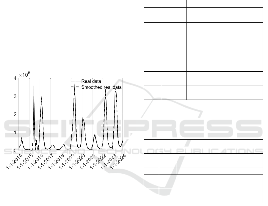
4 NUMERICAL RESULTS
In this section, the proposed model is validated con-
sidering as reference case the impact of dengue in
Brazil between January 1 2014 and January 1 2024,
(WHO, 2024b). The choice has been driven by the
fact that it is a case in which the epidemics produces
a not negligible number of infections and, at the same
time, a good surveillance policy is adopted, monitor-
ing the number of severe cases. The time history of
such a quantity is reported in Fig. 2; the original data
are plotted along with a version smoothed by means
of a Gaussian-weighted average of window 3.
Note a sort of periodicity, especially in the sec-
ond part of the time interval: a seasonality of about
12 months, with a peak of the severe cases occurring
every year in April corresponding, more or less, to the
last month of the more humid and warmer period.
Figure 2: Real cases of dengue epidemics in Brasil; con-
tinuous line: original real data, dashed line: smoothed real
data by a gaussian filter of window 3.
Some of the model parameters can be deduced
from dengue characteristics and herein assumed as
averaged quantities. What is known about dengue is
that, as said, in most cases, with mild symptoms, a
patient is recovered after about 2 weeks, whereas if
symptoms occur, usually beginning 4–10 days after
the infection, they last for a week. Most infected peo-
ple can transmit the virus for about 1 week, whereas
the presence of viral particles in the blood (viremia)
can last up to 12 days. The mortality rate due to se-
vere cases is about 5%, but if not treated it can reach
20%.
Actually, dengue disease can be caused by one of
the 4 viruses, Den-1, Den-2, Den-3, Den-4, allowing
to get immunization only for the specific family that
has infected the patient; here, in order to maintain the
model as simple as possible, this distinction is not im-
plemented, favouring an average human population
behaviour with respect to infection and introducing
the possibility to be reinfected.
As far as the parameters regarding the human pop-
ulation, the values in Table 1 are taken.
Table 1: Values of the parameters of human population used
in the numerical simulations.
d
S
H
10
−6
from statistic data
d
I
H
10
−6
from statistic data
d
R
H
10
−6
from statistic data
d
I
HF
5 · 10
−6
illness statistics
γ
I
H
1 one month for recovery
for asymptomatic individuals
γ
HF
1/3 three months for recovery
for symptomatic individuals
r 1/2 two months of immunity
before possible reinfection
A
H
50 population characteristics
(see S
e1
H
)
α 0.99 only 1% of infected
has severe consequences
As far as the parameters regarding the vector pop-
ulation, the values in Table 2 are chosen.
Table 2: Values of the parameters of vector insect popula-
tion used in the numerical simulations.
d
S
V
1/3 3 months of life for uninfected
insects
d
I
V
1/3 3 months of life for infected
insects
a 1/4 4 months as reproduction time
A
V
10
6
population characteristics
(see S
e1
V
)
ϕ 0.01 99% of severely infected patients
assumed recovered and protected
The two parameters β
HV
and β
V H
are, respec-
tively, the transmission rates between healthy hu-
mans S
H
and the infected vectors I
V
and between the
healthy vectors S
V
and the infected humans, I
H
or I
HF
.
They represent the average rate at which an infected
individual (mosquito / human) can infect a suscepti-
ble one (human / mosquito); they depend mainly on
the specificity of the epidemic disease, that is on the
probability of infection on contact, on the number of
contacts of an infected patients, on the infectious ca-
pability of the insects, and on the robustness of the
individuals with respect to the contact with the virus.
As already stated in the Introduction, the dengue
epidemic is a disease whose seasonality spread is
strongly dependent on the reproduction cycle of the
vectors; this justifies the periodicity of about 12
Modelling and Analysis of Spread Characteristics of Arbovirus Infections
607

months that can be noted in dengue spread in the case
study analysed, Fig. 2.
The insect population dynamics here considered is
a basic description that do not explicitly include any
season dependency and then the periodicity in their
life cycle is not present. A more sophisticated model
could considers these factors, but in this preliminary
study the time changes in the insect effects on the dis-
ease are modeled as time dependent values of β
HV
and
β
V H
. This allows to describe the different stages of
dengue spread that increases during the warmer and
more humid months, followed by a fast decrease in
autumn and winter. Then, they are not prefixed, but
dependent on the epidemic evolution. For this rea-
son, they are determined on the basis of the available
data, by minimizing the error between the real data I
R
and the corresponding output of the model I
HF
; this
quantity is described by means of two terms, the sum
of the square of the errors, month by month, and the
maximum of the difference of the errors:
J(β
HV
,β
V H
) =
R
t
f
t
i
w(I
R
− I
HF
)
2
+ max(I
R
− I
HF
) (68)
being w a weight chosen equal to 10
−3
, used to nor-
malize the two elements of the cost index.
The minimization is obtained in the time inter-
val corresponding to [t
i
t
f
] to be chosen inside the
period in which the real data are available. Two
main intervals of 6 months are considered every 12
months: November- April and May-October, cor-
responding for the Southern Hemisphere to spring-
summer and autumn-winter, respectively; every 6
months, a unique value of each of the transmission
rates β
HV
and β
V H
is estimated.
The results are obtained by applying the optimiza-
tion algorithm of interior-point, that approximates the
Hessian using finite differences.
To avoid data inconsistency, in the following the
interval October 1 2020 December 1 2023 is consid-
ered.
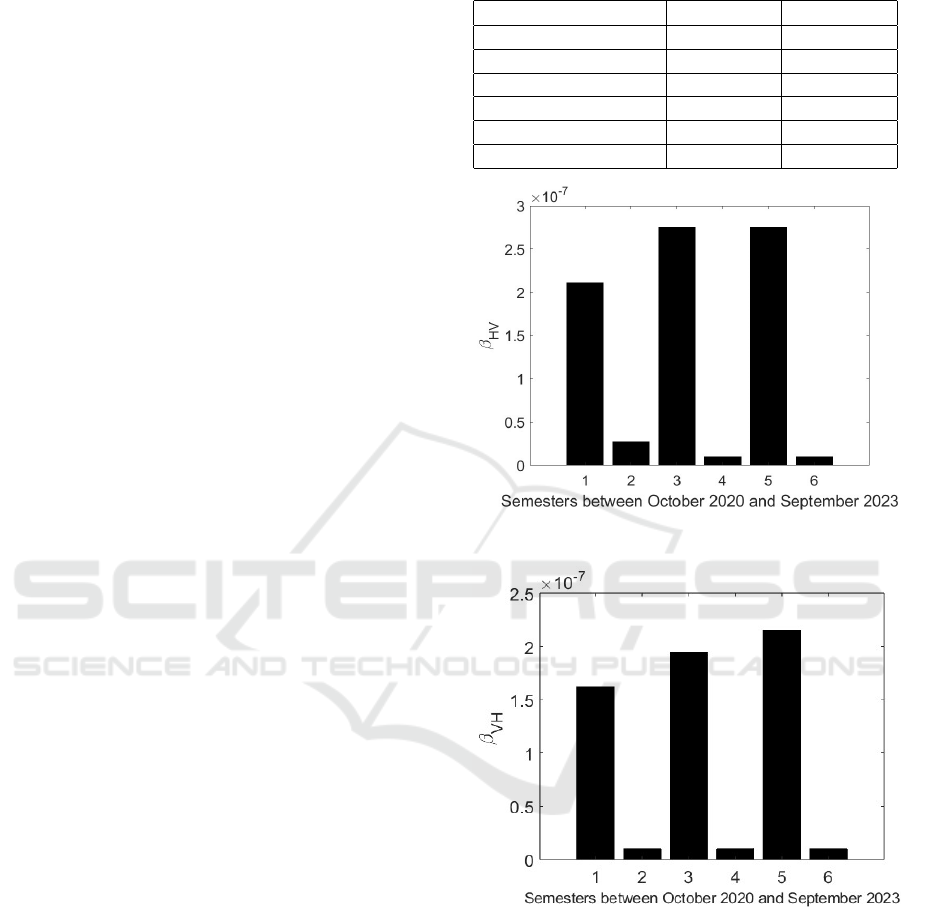
Results are reported in Table 3; in Figs. 3 and 4
the behaviors of the transmission rates β
HV
and β
V H
are shown respectively. Note the high values corre-
sponding to the semester of spring-summer in Brasil
and the lower ones in the semester corresponding to
autumn and winter.
To show the effectiveness of the identification pro-
cedure and of the proposed modelling, the recon-
structed state I
HF
, obtained by using the identified
values of the transmission rates, is plotted in Fig.5
with the true evolution I
R
referring to the period Octo-
ber 1, 2020 and December 1, 2023: a good correspon-
dence of the values and the general seasonality trend
can be observed.
As expected, in the period in which the spread
increases the identified transmission rates have the
Table 3: Values of transmission rates β
HV
and β
V H
.
Semester β
HV
(10
−6
) β
V H
(10
−6
)
10/01/20 – 3/1/21 0.211 0.162
04/01/21 – 9/1/21 0.027 0.010
10/01/21 – 3/1/22 0.275 0.195
04/01/22 – 9/1/22 0.010 0.010
10/01/22 – 3/1/23 0.274 0.215
04/01/23 – 9/1/23 0.010 0.010
Figure 3: Transmission rate β
HV
in the 6 semesters starting
on October 2020.
Figure 4: Transmission rate β
V H
in the 6 semesters starting
on October 2020.
highest values; as mentioned, the expedient adopted
allows to highlight the seasonality of the epidemic due
to dengue as if the latter depended on the greater or
lower contagiousness of mosquitoes and not on their
normal reproductive cycle.
The availability of a validated model allows to per-
form some analysis of the disease characteristics. For
example, it is possible to take into account one of
the most common parameter, which provides indica-
tions on the spread of the infection, the reproduction
number, as discussed in Subsection 3.3; in particular,
ICINCO 2024 - 21st International Conference on Informatics in Control, Automation and Robotics
608

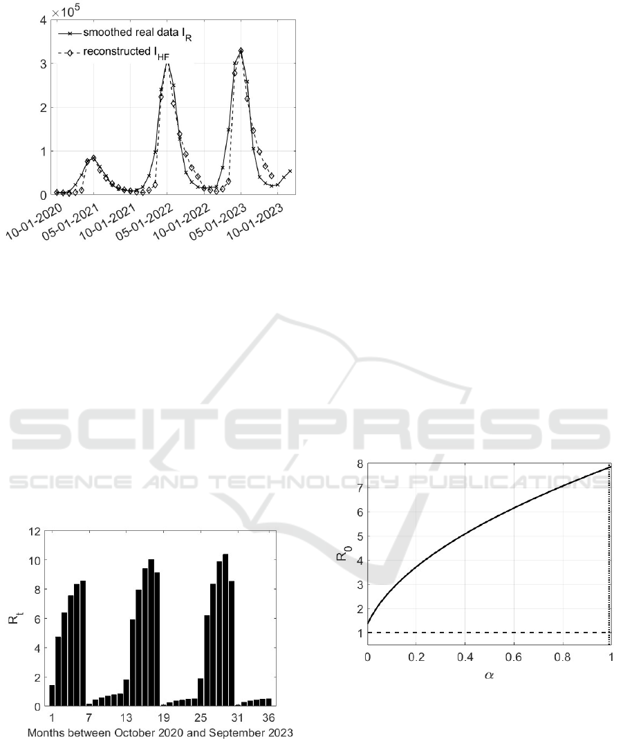
Figure 5: Example of the effectiveness of the reconstruction
of the number of severe infected patients by using the iden-
tified values of the transmission rates in the period October
2020 - December 2023.
during the epidemic spread, the most meaningful is
R
t
, whose expression has been computed in Subsec-
tion 3.3 and reported in (62). It is now possible to
evaluate it by using the monthly values of suscepti-
ble individuals and vectors. This implies that a value
of R
t
can be calculated for each month; the results
are reported in Fig. 6. In the months in which the
dengue spread increases, the corresponding R
t
has a
high value, that rapidly decreases in the successive
months. The rapid decrease of this indicator depends
mainly on the changed environmental conditions for
the vectors, ascribed in the present modelling, to the
transmission rates.
Figure 6: Reproduction number R
t
evaluated monthly be-
tween October 2020 and September 2023.
It is interesting to study the influence on the ba-
sic reproduction number of some parameters, also in
view of the application of possible prevention and
containment measures. In particular, the most rel-
evant parameters will be varied, keeping the others
constant and equal to the values already introduced.
In Fig. 7, note that the basic reproduction number
R
0
increases with α, starting, with the chosen values
of the other parameters, at R
0
= 1.3596 > 1. This im-
plies that a population with a reduced number of pa-
tients with severe symptoms cannot by itself decrease
the spread: the less are the asymptomatic individuals,
the more slow is the epidemic spread, but the infec-
tion increases anyway.
Similar consideration can be applied studying the
influence of the growth parameter a on R
0
; in Fig.8
it can be noted that, as reasonable, R
0
increases with
parameter a; also in this case the reduction of the only
reproductive capability of mosquitoes is not sufficient
to reduce the basic reproduction number.
The dependence of R
0
to γ
HF
is reported in Fig. 9,
where a quite irrelevant contribution of the patients
recover parameter to the variation of the epidemic
spread is evidenced.
Different considerations can be referred to the
death rates of mosquitoes, d
SV
= d
IV
, Fig. 10. In this
case the influence is evident: by increasing this value
(for example by suitable disinfestation campaign on
the eggs or larval individuals) it is possible to reduce
the R
0
up to values lower than 1. In this simulation,
keeping the same values for all the other parameters,
but increasing d
SV
= d
SV
> 1.46, it is possible to ob-
tain R
0
< 1.
Figure 7: Variation of the basic reproduction number R
0
with respect to α.
5 CONCLUSIONS
Climate changes and increased movements of people
and goods are making arboviruses a new epidemic
emergency all over the world. Generally, human pop-
ulation does not suffer severe symptoms, but a sig-
nificant percentage of patients can even die for the
Modelling and Analysis of Spread Characteristics of Arbovirus Infections
609

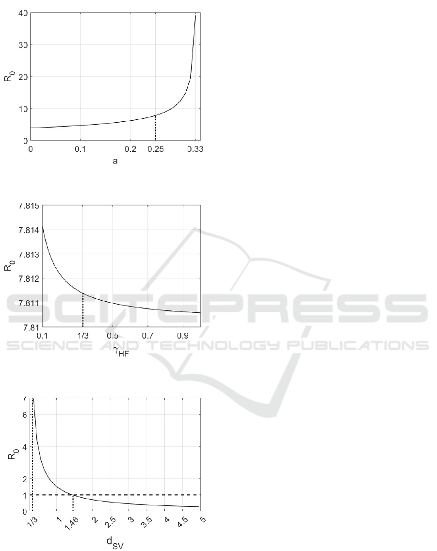
Figure 8: Variation of the basic reproduction number R
0
with respect to a.
Figure 9: Variation of the basic reproduction number R
0
with respect to γ
HF
.
Figure 10: Variation of the basic reproduction number R
0
with respect to d
SV
.
consequences of such infections, also for the absence
of specific medication. The arboviruses have an in-
trinsic seasonality, due to the environmental require-
ments for mosquitoes’ reproduction and survival. In
this paper, making use of compartmental modeling
framework, it is proposed and analysed a new model
in which human and mosquitoes populations interact,
infecting each other; the conditions for the existence
of a disease free equilibrium point and the endemic
one are determined, along with the basic and current
reproduction numbers.
The model is validated by using recent data of
dengue disease from Brazil, showing the seasonality
aspect of this epidemic and discussing the influence
of the model parameters on the disease evolution, also
to model future lines of intervention for effective pre-
vention and containment measures.
ACKNOWLEDGEMENTS
The Authors wish to thank the Istituto Nazionale di
Alta Matematica Francesco Severi in Rome for its
support.
REFERENCES
Abidemi, A., Fatmawati, and Peter, O. (2024). An opti-
mal control model for dengue dynamics with asymp-
tomatic, isolation, and vigilant compartments. Deci-
sion analytics Journal, 100413:1–20.
Alutto, M., Cianfanelli, L., Como, G., and Fagnani, F.
(2024). On the dynamic behavior of the network sir
epidemic model. IEEE Transactions on Control of
Network Systems, pages 1–12.
Arquam, M., Singh, A., and Cherifi, H. (2020). Impact of
seasonal conditions on vector-borne epidemiological
dynamics. IEEE Access, 8:94510–94525.
Attaullah, A. and Sohaib, M. (2020). Mathematical model-
ing and numerical simulation of HIV infection model.
Results in Applied Mathematics, 7:1–11.
Ayele, T., Goufo, E., and Mugisha, S. (2021). Mathematical
modeling of HIV/AIDS with optimal control. Results
in Physics, 26(104263):1–14.
Barcellos, C., Matos, V., Lana, R., and Lowe, R. (2024).
Climate change, thermal anomalies, and the recent
progression of dengue in brazil. Scientific Reports,
14(5948).
CDC (2024). Center for disease control and prevention.
https://www.cdc.gov/.
Di Giamberardino, P., Compagnucci, L., De Giorgi, C.,
and Iacoviello, D. (2019). Modeling the effects of
prevention and early diagnosis on hiv/aids infection
diffusions. IEEE Transactions on Systems, Man, and
Cybernetics: Systems, 49(10):2119–2110.
Di Giamberardino, P. and Iacoviello, D. (2017). Optimal
control of SIR epidemic model with state dependent
switching cost index. Biomedical Signal Processing
and Control, 31:377–380.
ICINCO 2024 - 21st International Conference on Informatics in Control, Automation and Robotics
610

Di Giamberardino, P. and Iacoviello, D. (2021). Evaluation
of the effect of different policies in the containment of
epidemic spreads for the COVID-19 case. In Biomed-
ical signal processing and control. Elsevier.
Di Giamberardino, P., Iacoviello, D., Papa, F., and Sinis-
galli, C. (2021). A data-driven model of the covid-19
spread among interconnected populations: epidemio-
logical and mobility aspects following the lockdown
in italy. Nonlinear Dynamics, 106(2):1239–1266.
Diagne, M. L., Rwezaura, H., Tchoumi, S. Y., and
Tchuenche, J. M. (2021). A mathematical model of
COVID-19 with vaccination and treatment. Com-
putational and Mathematical Methods in Medicine,
(1250129):1–16.
Schaum, A., Bernal-Jaquez, R., and G.Sanchez-Gonzales
(2022). Model-based monitoring of dengue spreading.
IEEE Access, 10:126892–126898.
Sow, A., Diallo, C., and Cherifi, H. (2024). Interplay be-
tween vaccines and treatment for dengue control: an
epidemic model. PLOS ONE, pages 1–27.
Van Den Driessche, P. (2017). Reproduction numbers of
infectious disease models. Infectious disease model-
ing, 2(3):4770–4777.
WHO (2024a). https://www.who.int/.
WHO (2024b). Dengue-Global Situation.
https://www.who.int/emergencies/disease-outbreak-
news/item/2024-DON518.
Xu, C., Xu, J., and Wang, L. (2024). Long-term effects of
climate factors on dengue fever over a 40-year period.
Public Health, 24(1451):1–11.
Yi, C., Cohnstaedt, L., and Scoglio, C. (2021). Seir-sei-
enkf: a new model for estimating and forecasting
dengue outbreak dynamics. IEEE Access, 9:156758–
156767.
Zhu, X., Gao, B., Zhong, Y., Gu, C., and Choi, K. (2021).
Extended kalman filter based on stochastic epidemio-
logical model for covid-19 modelling. Computers in
Biology and Medicine, 137(104810):1–10.
Modelling and Analysis of Spread Characteristics of Arbovirus Infections
611