Autonomous Forklift Navigation Inside a Cluttered Logistics Factory
Eric Lucet
a
, Antoine Lucazeau and Jason Chemin
Universit
´
e Paris-Saclay, CEA, List, F-91120, Palaiseau, France
Keywords:
Autonomous Navigation, Road Network, Local Planning, Path Tracking, Obstacle Avoidance, Forklift Space
Constraints.
Abstract:
This paper presents the complete architecture of an application for autonomous forklift navigation in the
cluttered and changing environment of a printing factory. A global path is selected from an existing road
network, based on available navigation tracks. Then, a local path planner coupled with a path-following
controller enables the navigation of the autonomous robots. A finite-state machine (FSM) architecture ensures
transitions between the different operating modes of a robot during a mission, including obstacle avoidance.
Navigation corridors are dynamically defined and are respected through the definition of tracking control
constraints, enabling safe and efficient navigation at all times, taking into account the space constraints of a
forklift truck in a congested factory. A forklift robot and its environment were simulated in ROS Gazebo to
validate the approach, before carrying out in-depth experiments on a real robot prototype and estimating its
performance in real-time during realistic operational scenarios.
1 INTRODUCTION
The French OTPaaS institutional project brings to-
gether academic and industrial partners to tackle in-
novative industrial use cases, particularly the automa-
tion of load transport in a printing plant. Achieving
this task requires the autonomous navigation of mo-
bile robots, which presents challenges in cluttered en-
vironments and in the presence of operators. More-
over, a particularity of forklift systems designed for
such use cases (Ilangasinghe and Parnichkun, 2019)
is that the forks occupy a significant amount of space
at the rear of the vehicle, which can result in large
displacements when the vehicle rotates. Additionally,
such forks are used for precise picking maneuvers,
and also precise navigation is needed to avoid static
or dynamic obstacles, as well as accounting for the
space requirements of a forklift truck, for safety rea-
sons. At the same time, optimizing the trajectory to be
followed in terms of length, duration and smoothness
can improve logistical activity.
1.1 Use Case Description
The main goal of this scenario of load transporta-
tion in a factory is to move a paper bin from site A
a
https://orcid.org/0000-0002-9702-3473
to B, while complying with numerous industrial con-
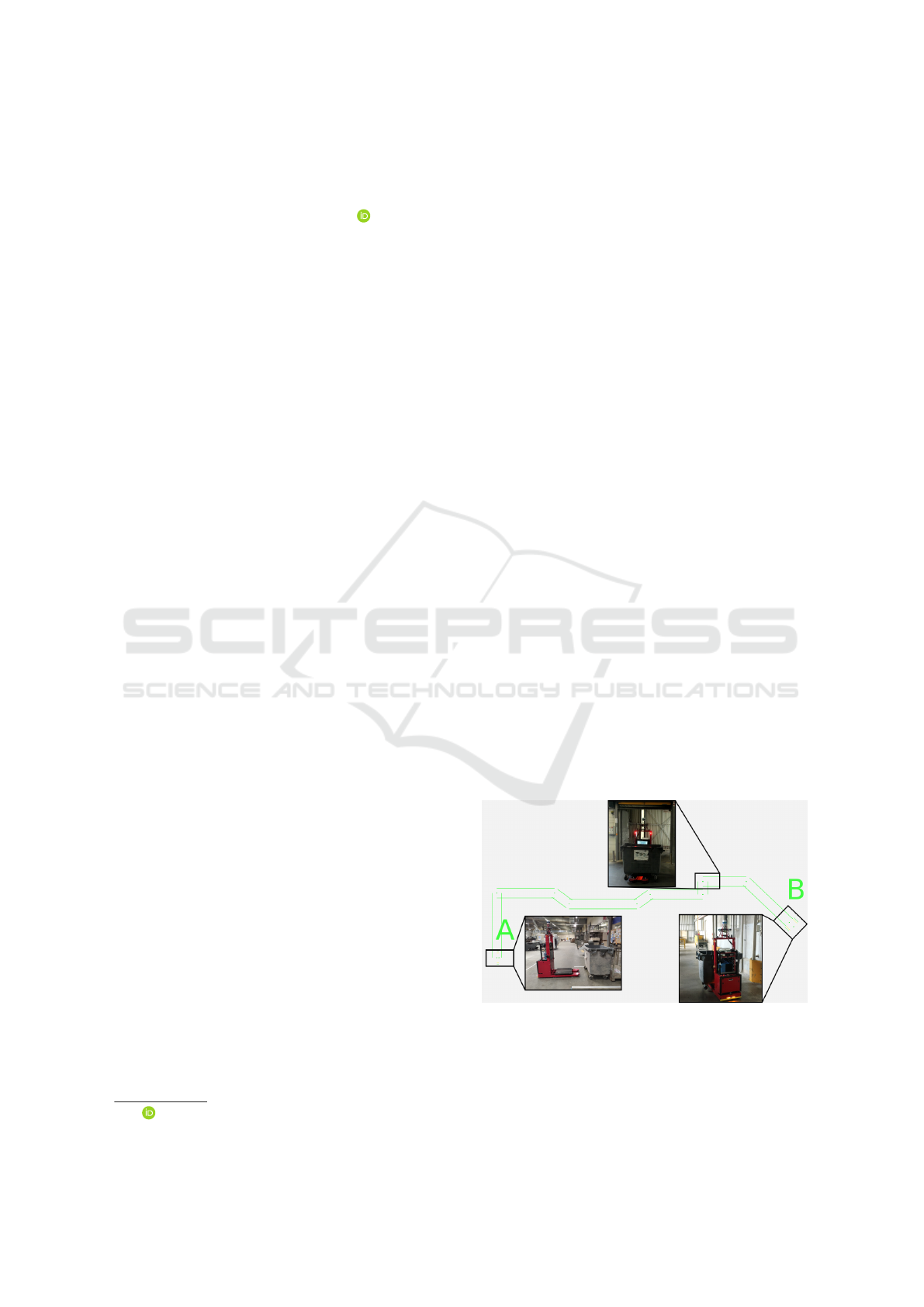
straints. An example of this use case is illustrated in
Figure 1. This illustration shows the robot position-
ing itself accurately in front of the paper bin at site A,
loading it onto its forks, moving it through various en-
vironments and several doors, and finally depositing it
at site B. Throughout this process, particular attention
is required to maintain the stability of the container
and ensure the safety of its surroundings as the robot
will have a larger footprint and be more encumbered.
Figure 1: Different stages during use case realization.
The autonomous robot prototype displayed is a
TwinswHeel facTHory forklift droid designed specif-
ically for the OTPaaS project. This mobile robot is
a differentially steered vehicle, equipped with two
Lucet, E., Lucazeau, A. and Chemin, J.
Autonomous Forklift Navigation Inside a Cluttered Logistics Factory.
DOI: 10.5220/0013067600003822
Paper published under CC license (CC BY-NC-ND 4.0)
In Proceedings of the 21st International Conference on Informatics in Control, Automation and Robotics (ICINCO 2024) - Volume 2, pages 327-335
ISBN: 978-989-758-717-7; ISSN: 2184-2809
Proceedings Copyright © 2024 by SCITEPRESS – Science and Technology Publications, Lda.
327

large, centered drive wheels and four small caster
wheels at the corners of the front chassis for stabil-
ity. It navigates through predefined straight corri-
dors, defined by two real or virtual walls, and must
remain strictly within their boundaries to ensure the
safety of nearby employees. To further ensure safety,
collision avoidance is crucial, and smooth control is
preferred to make the robot’s behavior predictable to
those around it. Additionally, the environment may
also present dynamic challenges, such as blocked cor-
ridors or the presence of other vehicles. While a pre-
existing global map is available, dynamic elements
need to be updated via SLAM using Lidar and vision
systems.
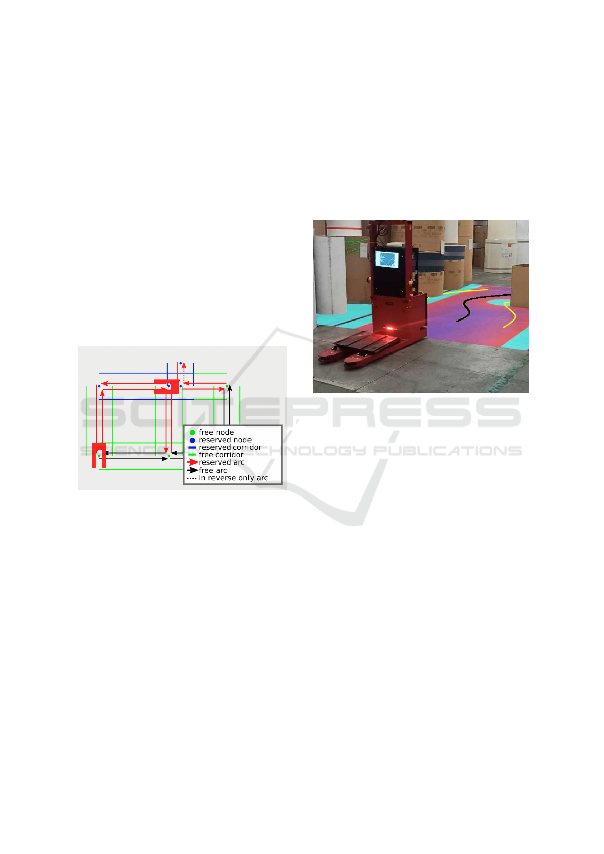
Given the structured nature of the environment, a
directional-graph-based approach is chosen for global
navigation, with nodes representing corridor intersec-
tions and edges representing the corridors themselves
(see Figure 2). The application has to be able to man-
age multiple autonomous forklifts sharing corridors
with each others.
Figure 2: Example of multi-robot path planning.
For local navigation, a custom solution is imple-
mented with specific safety constraints tailored to the
scenario. For that, local navigation is separated into
two tasks: a local path planning algorithm is used
over a costmap, and a path tracking controller is im-
plemented. The choice of such algorithms and their
implementations are described in the following.
1.2 Navigation Strategies
The objective in robotic navigation is to move in a
feasible manner, avoiding obstacles, while minimiz-
ing costs such as path length or computational time.
Similar to human reasoning, navigation can operate
on different scales: selecting the optimal route at a
high level (e.g., choosing streets) and managing ob-
stacle avoidance at a more granular level (e.g., navi-
gating in it, avoiding pedestrians).
While it is theoretically possible to compute an
optimal path by considering all these factors simul-
taneously, this approach leads to exponential compu-
tational growth. Such complexity can make planning
towards a distant target prohibitively time-consuming.
To address this, a divide-and-conquer strategy is often
employed, separating the problem into Global Navi-
gation (path planning) and Local Navigation (obsta-
cle avoidance, motion planning, path tracking) (Fox
et al., 1997; Chemin, 2022).
Figure 3: Forklift robot navigating in the printing plant.
Global Planning Methods. To find key waypoints
to reach sequentially at a higher level, existing so-
lutions include graph-based, mesh-based, sampling-
based such as PRM (Bohlin and Kavraki, 2000) and
RRT (Karaman et al., 2011), and grid-based ap-
proaches. Though computationally intensive, these
methods are acceptable for low-frequency calls.
Local Planning Methods. Once waypoints are iden-
tified through global planning, local methods are used
to connect these points with feasible paths for the
robot to follow. These paths must consider kine-
matic and dynamic constraints while ensuring colli-
sion avoidance. Key criteria here include speed and
reactivity, as these methods must be called frequently.
Interpolation techniques such as B
´
ezier curves or B-
splines are effective but can struggle with obstacle
avoidance, often requiring optimization-based solu-
tions (Choi et al., 2008). Popular local methods in-
clude Dynamic Window Approach (DWA) (Fox et al.,
1997) which is sampling-based, and Timed Elastic
Band (TEB) (R
¨
osmann et al., 2012), or more gener-
ally, Model Predictive Control (MPC) (Wang et al.,
2019; Weber and Gerdes, 2023) which solve opti-
mization problems to find paths that respect given
constraints. Potential field methods, coupled to clas-
sical search algorithm such as A*, can be used to repel
from obstacles and attract the robot towards a distant
ICINCO 2024 - 21st International Conference on Informatics in Control, Automation and Robotics
328

goal (Meng and Fang, 2024). Finally, machine learn-
ing techniques also offer potential for generating fea-
sible paths in unknown and harsh environments (Josef
and Degani, 2020).
Path Tracking Methods. Some methods mentioned
above generate paths, but may not provide direct
control commands to the robot for following these
paths (unlike TEB or DWA). In such cases, the local
navigation problem can be further divided into path
generation and path tracking control tasks. Several
path tracking techniques exist, including Pure Pur-
suit (Coulter, 1992), Stanley (Abdelmoniem et al.,
2020), PID (MS Saad and Darus, 2012), MPC (Wang
et al., 2019; Li et al., 2023), Sliding Mode Control
(Yang and Kim, 1999), and machine learning-based
approaches (Chemin et al., 2024).
Because of the dimensions of the nonholonomic
forklift robot, planning feasible paths for it in a clut-
tered space is difficult, similar to the “Piano Mover’s
Problem” (Schwartz and Sharir, 1983). Its forks are
susceptible to colliding with humans or objects as the
robot turns, presenting a serious danger. However,
the problem can be simplified in the given scenar-
ios, where the robot operates within predefined and
theoretically safe corridors. This limits its movement
and further reduces the risk of collision, making the
navigation problem more manageable and safer. In
the literature, several works propose technical im-
plementations relevant to the use case. Some stud-
ies present solutions for path planning, control and
self-localization of a forklift in a factory environment
(Tamba et al., 2009; Vivaldini et al., 2010). Addition-
ally, one study focuses on pallet detection, which is
crucial for the forklift to accurately identify, navigate
to, and handle the object (Syu et al., 2017).
Here, it was chosen to decompose the navigation
problem into: global path planning on graphs, local
path planning using A* over an obstacle costmap, and
finally a Constrained Linear Model Predictive Con-
troller (CLMPC) for path tracking, as displayed in
Figure 4. The path of the static graph of the road net-
work is followed in nominal navigation conditions, or
a dynamically generated path by the local planner is
followed when it is required for obstacle avoidance.
Figure 4: Application’s architecture.
1.3 Contributions
Main contributions are the following:
• A complete scenario, including accurate forward
and reverse navigation for picking up and setting
down loads, and obstacle avoidance with dynamic
definition of navigation corridors in a costmap.
• CLMPC path tracking algorithm handling specific
corridor constraints for a robot rectangle footprint.
• Integration of these components into a unified sys-
tem, their adaptation and evaluation in simulation
and real-world experiments.
Then, the paper is structured into 4 sections before
the conclusion. The second section presents the local
planner implemented. The third section presents the
path tracking controller used with the implementation
of lateral constraints. And the fourth section analyses
results achieved using the presented architecture.
2 LOCAL PATH PLANNING
2.1 Costmap
A costmap is a grid that assigns cost values to cells
based on traversal difficulty, guiding planners to opti-
mize safe and efficient paths.
The ROS costmap 2d package (Marder-Eppstein
et al., 2018) is a flexible tool used in robotic navi-
gation, allowing dynamic updates and customization
with multiple layers. The following layers are used:
• Obstacle Layer: Uses sensor data (e.g. Lidar) to
detect and track obstacles.
• Corridor Layer: Custom layer that defines virtual
corridors as obstacles to restrict navigation paths.
• Inflation Layer: Expands obstacles to create
safety buffers, with costs based on proximity and
the robot’s footprint, ensuring safe navigation.
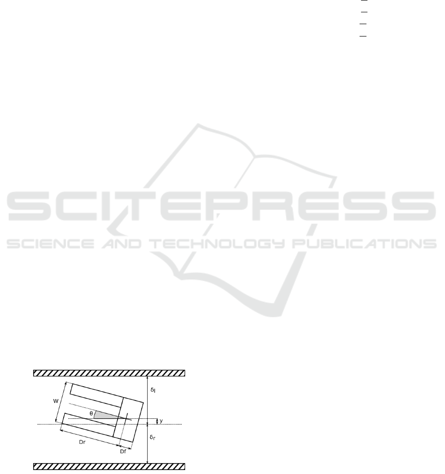
Given the inscribed radius r
inscribed
, that is the radius
of the largest circle that can be fully contained within
the robot’s footprint, as shown in Figure 6, we recall
that the inflation layer with scaling operates as fol-
lows: when the distance from the cell center to the
nearest obstacle d is less than r
inscribed
, the cell cost
is set to near maximum, cost
max
= 255. If the cell is
further than r
inscribed
, its cost decreases as the distance
d increases. This can be represented as:
cost = e
− f actor×max(0,d−r
inscribed
))
× (cost
max
− 1) (1)
In this work, the f actor controlling the rate of de-
cay is set to 1. This inflated representation of the
robot’s surrounding environment assists local plan-
ners in avoiding cells that are too close to obstacles.
In Figure 5, the costmap is visualized in shades
of red and blue, blue being a lower cost area. Pink
Autonomous Forklift Navigation Inside a Cluttered Logistics Factory
329

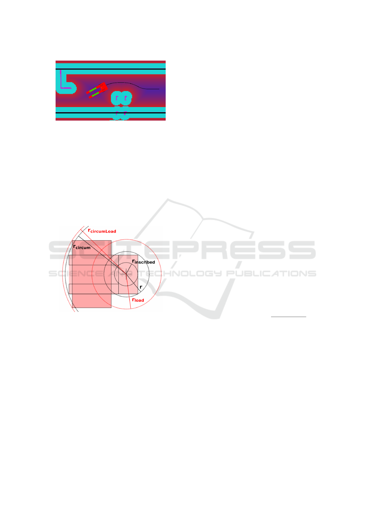
Figure 5: Avoidance scenario in a narrow corridor, with the
A* local path (black) and highlighted corridor walls (black).
cells are the physical location of obstacles that can be
real or virtual (such as corridors). Cyan cells corre-
spond to the inscribed radius of the robot’s footprint.
Both cyan and pink are Lethal cells which means the
control point of the robot cannot navigate over them
without a collision.
2.2 Simplified Corridor Navigation
A diagram of the robot, both with and without a load,
is shown in Figure 6.
Figure 6: Forklift robot and its inscribed and circumscribed
radiuses, starting from the wheelbase center, with and with-
out a load.
When unloaded, the costmap inflation distance
is set to a value within the range [r
inscribed
,r
circum
].
Choosing a distance equal to r
inscribed
does not fully
cover the robot’s lateral and longitudinal footprint,
which means the robot may be in collision at a given
cell position. Conversely, choosing r
circum
ensures
coverage of the whole robot, hence avoiding all pos-
sible collisions. However, this approach is overly
conservative, as it prevents the robot from navigating
through narrow corridors in the factory, such as the
scenario in Figure 5.
As an initial approximation, it is possible to con-
sider the small changes in the robot’s orientation dur-
ing navigation to compute a compromise value for r
between the inscribed and circumscribed radius. This
approach, while not fully secure and slightly conser-
vative, can provide a practical solution.
A more rigorous and less conservative solution is
to select a value for r that covers the robot’s width,
as illustrated in Figure 6, and then use the robot’s
rectangular footprint as a constraint in the tracking
controller. This approach addresses cases where the
robot’s orientation relative to the corridor is non-zero,
and the radius r alone is insufficient to model po-
tential collisions. The controller constraint ensures
that none of the four corners of the rectangle defin-
ing the robot’s footprint collides with any obstacle.
This method prevents the loss of navigation solutions
in narrow corridors. A similar approach can be ap-
plied when the robot is under load, where both r and
the constraint need to be adjusted accordingly.
2.3 A* Path Search Configuration
A classical and efficient A* search is used on the
costmap to compute local paths. Given a distant way-
point from the global path planner, the local planner’s
task is to generate a collision-free path towards this
waypoint. The waypoint is used if it is reachable
within the local costmap. Otherwise, a sub-target is
selected within a low-cost cell in the corridor, ensur-
ing it is accessible. The costmap specifies safe and
collision-free cells, and the objective is to find the
shortest path through the corridor to the target while
maintaining a safe distance from obstacles, as illus-
trated in Figure 5.
Heuristics. The heuristic is based on the Manhattan
distance between the robot’s starting position and the
sub-target. This distance is then scaled by the average
cost of the start and end cells, s and e, in the costmap:
h = (|s.x − e.x| + |s.y − e.y|) ∗
s.cost + e.cost
2
(2)
This approach provides a simple and fast heuristic that
considers both the path distance and an estimate of its
cost. Although this formula can potentially overesti-
mate the cost in certain situations, other heuristic de-
signs are planned for future improvements. Despite
this, it was empirically shown that this heuristic per-
formed well in most scenarios, significantly reducing
the number of search iterations compared to a classi-
cal Dijkstra algorithm (h = 0).
Pathfinding Strategies. The A* used in this work
implements multiple strategies to enhance exploration
and ensure safe path generation. First, it prevents
paths to traverse costmap cells exceeding a prede-
fined threshold. This threshold is calculated before-
hand using the desired safe distance to obstacles, as
per Eq. (1). Next, exploration is restricted to the tar-
get direction, focusing only on forward exploration
ICINCO 2024 - 21st International Conference on Informatics in Control, Automation and Robotics
330

within the corridor. This prevents inefficient or coun-
terproductive backward movements. While the algo-
rithm usually explores neighboring cells horizontally
and vertically, incorporating diagonal movements in
the target direction reduces iterations and produces
smoother paths. While it may conflict with Manhat-
tan distance-based heuristics, we chose to add diago-
nal movements to enhance path smoothness. A* algo-
rithm terminates when it finds a path within the corri-
dor that reaches a region near the local end goal. Fi-
nally, a box blur smoothing technique is applied to
refine the path before providing it to the controller.
3 PATH TRACKING
This section describes the implementation of a model
predictive controller (MPC) based on the kinematic
model of the differential steer robot. MPCs have been
extensively utilized in mobile robotics due to their
ability to handle constraints and predict future system
behavior (Yakub and Mori, 2013; Oyelere, 2014). In
the study by (Ji et al., 2017), the authors employ a
discrete linear model for vehicle lateral and yaw dy-
namics, assuming a constant longitudinal velocity, to
achieve collision-free navigation along a given path.
Here, a Constrained Linear Model Predictive Con-
trol (CLMPC) algorithm is derived from (Lucet et al.,
2021), to be adapted to a differential steer robot. The
robot kinematic model is linearized by considering a
navigation path of constant curvature c
m
. As a result,
predicted states are computed as follows:
Y = Ay
0
+ BU + C (3)
In Eq. (3), state matrices A and B are defined with
O and 1 values, U is the control vector and C is de-
fined from curvature values c
m
at sampling steps ab-
scissas of the control spacial horizon. By using this
equation, a quadratic function of the predicted error
state Y and of the future control input U is optimized.
Figure 7: Robot parameters in a corridor.
Then, state constraints are expressed by consider-
ing the four corners of the vehicle footprint approxi-
mated as a rectangle with front and rear ends at a dis-
tance of D
f
and D
r
respectively from the control point
along the longitudinal axis, with W its width along the
lateral axis, and θ its orientation relative to that of the
reference path (see Figure 7). Setting these four cor-
ners to remain within a tolerance δ
l
to the left of the
path and δ
r
to the right of the path, can be written as
follows:







−δ
r
< y +D
f
sinθ −
W
2
cosθ < δ
l
−δ
r
< y +D
f
sinθ +
W
2
cosθ < δ
l
−δ
r
< y −D
r
sinθ −
W
2
cosθ < δ
l
−δ
r
< y −D
r
sinθ +
W
2
cosθ < δ
l
Then, by linearizing for small values of θ, it results:
Dy + d ≥ 0
8×1
(4)
In Eq. (4), matrix D is defined with D
f
and D
r
values, and matrix d is defined with W , δ
l
and δ
r
val-
ues. To compensate for any linearization errors, D
f
,
D
r
and W values are slightly increased (≈ 4%) as a
function of maximum θ value.
Extended to all the n predicted states of the con-
troller and written as a function of future controls by
using Eq. (3), the constraint is finally expressed as fol-
lows:
DBU + d
gap
+ DAy
0
+ DC ≥ 0
8n×1
(5)
with:
• D, a block diagonal matrix of n blocks D;
• d
gap
, a block column matrix of n blocks d.
Various factors can have an impact on constraint
compliance, such as variable longitudinal velocity,
state estimation errors, model errors, or variable cur-
vature. To reduce these inaccuracies, one solution is
to shorten the prediction horizon. It is also useful to
reduce the sampling step, which increases controller
accuracy. At the same time, this also increases the
size of the matrices and thus the computations re-
quired, hence the possibility of considering a variable
step size to respect a constraint without increasing the
computations, as proposed by (Lamburn et al., 2014).
Then, CLMPC outputs the robot yaw spatial
derivative setpoint. This control output is multiplied
with the robot’s longitudinal speed, determined by a
separate algorithm taking into account factors such as
path curvature and environmental risk. The resulting
yaw rate is sent to the robot’s low-level controller.
For example, Figure 8 displays path tracking plots
with an initial lateral error of 1m, for different lateral
tolerance constraints. Such constraints restrict the al-
lowable angular error amplitude for correcting lateral
deviations, thereby reducing the lateral error conver-
gence rate.
Autonomous Forklift Navigation Inside a Cluttered Logistics Factory
331

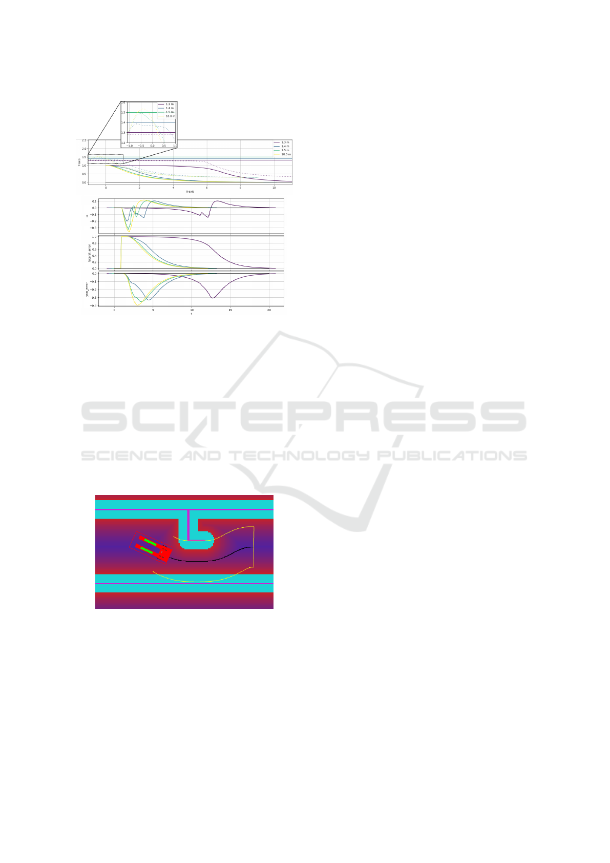
Figure 8: Path tracking for different lateral tolerance con-
straints.
Dynamic Corridor Constraints. These constraints
ensure the robot stays within a certain distance of the
local path, which can be visualized as a dynamic cor-
ridor within the user-defined virtual corridor, shown
in yellow in Figure 9. By enforcing these constraints
in the CLMPC, the robot’s front and rear ends are pre-
vented from crossing the corridor’s boundaries, ac-
counting the robot’s dimensions. This approach al-
lows the robot to temporarily deviate from the path if
necessary, to ensure it always stays within the desired
corridor. In the absence of obstacles, the constraints
align with the nominal static corridor walls.
Figure 9: Obstacle avoidance in a corridor, with the robot
footprint (red rectangle), the A* local path (black), and the
dynamic corridor (yellow) for CLMPC.
Predictive Safety Stop. Because the CLMPC oper-
ates over a certain prediction horizon, it can detect any
unsolvable situations ahead of time. In such cases, to
enhance safety, the robot anticipates the risk of a col-
lision and stops immediately to avoid it.
4 RESULTS
4.1 Test Specifications
Real-world experiments were performed using a
robotic prototype in a functioning printing factory. In
these tests, the robot began at the start of a 20m long
corridor and navigated forward by perceiving obsta-
cles, generating a costmap, planning a collision-free
local path with A* or TEB, and computing the nec-
essary controls with CLMPC to follow the path while
respecting corridor constraints. Additional obstacles
were introduced to simulate more complex environ-
ments. The robot, an autonomous forklift, measures
137cm in length, 80cm in width, and 176cm in height,
with an unloaded weight of approximately 120kg.
4.2 Results Analysis
4.2.1 CLMPC Gain Tuning
For control tuning experiments, robot localization is
ensured solely by wheel odometry, so as not to intro-
duce additional errors due to position readjustment in-
duced by exteroceptive sensors, Lidar or camera. The
robot moves in a straight line in a corridor 20m long
and 3m wide, with an initial lateral error of 1m. It
is operated at a speed of 1m/s with a control horizon
of 2m. CLMPC gains tuned are k
p
, which influences
the magnitude of lateral error correction, and k
d
, the
orientation error correction. Each set of parameters is
tested several times.
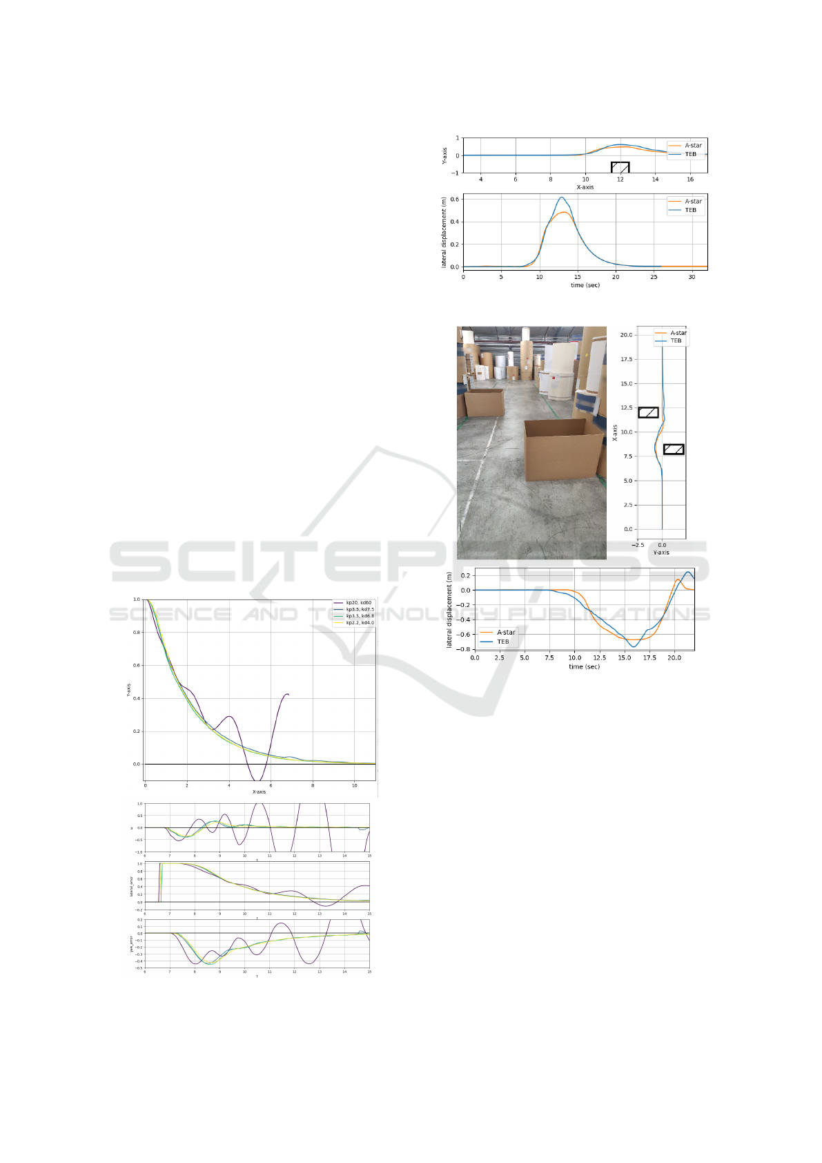
Figure 10 displays the results obtained during this
tuning process. Gains were evaluated based on the
robot convergence to the center of the corridor, as
measured by both lateral and yaw errors. For gains of
k
p
= 20.0 and k
d
= 60.0, the robot exhibits oscillatory
behavior and fails to converge in any of the assessed
metrics. Among the other tested gains, k
p
= 2.2 and
k
d
= 4.0 were selected, as they provide the fastest
convergence of both yaw and lateral errors to zero
while avoiding oscillatory yaw rate control output.
4.2.2 Local Path Planning
Simulations and real-world experiments were con-
ducted using the customized A* and TEB local path
planning algorithms to compare their performance.
Tests were conducted in three distinct scenarios:
one in which the robot had to avoid a single obstacle
positioned on the right side of the corridor (see Fig-
ure 11), one where the robot was required to navigate
through a chicane with two obstacles on the oppo-
site sides of the corridor (see Figure 12), and another
ICINCO 2024 - 21st International Conference on Informatics in Control, Automation and Robotics
332

where the robot navigated through two consecutive
obstacles on the same side of the corridor (see Figure
13). Additionally, for safety reasons, the robot’s lon-
gitudinal speed was modulated according to the path
curvature, resulting in fluctuations.
To measure the performance of the two local path
planners, the following metrics are considered.
• distance traveled : the total distance of the path the
robot has traveled while avoiding the obstacle;
• Time in avoid state : the duration the robot took
to avoid the obstacle;
• Energy expended : the kinetic energy expanded
by the robot, following the model presented by
(Liu and Sun, 2014):
Z
t
(m∗max{v(t)a(t),0}+I ∗max{ω(t)β(t),0})dt
• cumulative yaw : the following sum:
∑
|
dyaw
|
These metrics primarily assess the efficiency of
the various paths generated by the planners and their
suitability for integration with the selected controller.
Results are displayed in Table 1. Overall, A*
outperforms TEB, with the exception of the real test
with the obstacle on the right side of the robot’s path,
Figure 10: Path tracking for different CLMPC gain values.
Figure 11: Single-obstacle path tracking using A* or TEB.
Figure 12: Chicane path tracking using A* or TEB.
where A* takes more time to finish than TEB, but
anticipates the obstacle better with a smoother pro-
posed path. Other metrics in which A* consistently
outperforms TEB are total distance travelled and cu-
mulative angle. The performance gap between the
two path planners is significant for the chicane exper-
iments where TEB struggled. It should also be noted
that simulated and real experiments show comparable
results, when the algorithm used returns a solution.
Furthermore, comparing trajectories using A* or
TEB, the following results are obtained. TEB’s path
is less smooth with a greater amplitude of lateral dis-
placement than that of the A*. When the robot fol-
lows the TEB path, the total distance covered to avoid
the obstacle is generally greater. In addition, TEB
paths are more likely to fluctuate over the CLMPC
horizon, as illustrated by the experimental result in
Figure 12, which limits its tracking performance. The
Autonomous Forklift Navigation Inside a Cluttered Logistics Factory
333

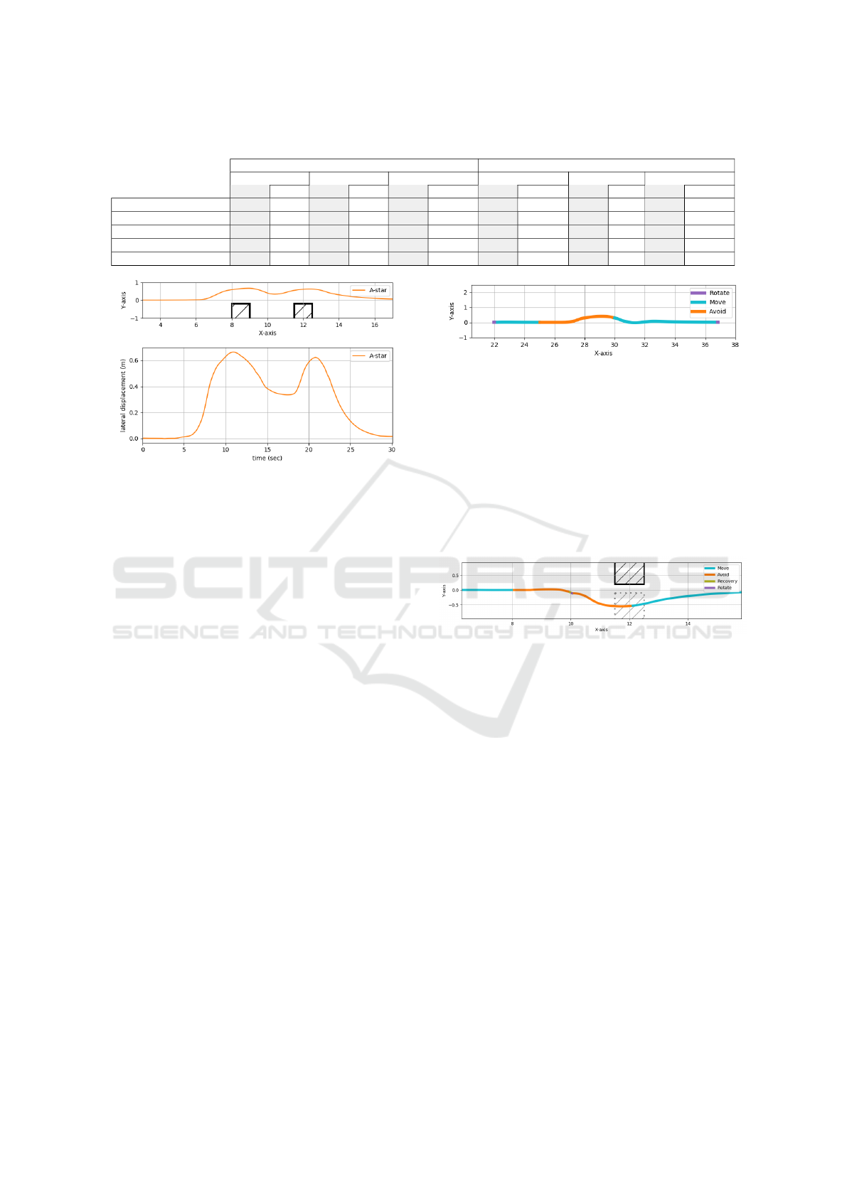
Table 1: Experimental results.
Simulated Real
right obstacle chicane 2x right obstacle right obstacle chicane 2x right obstacle
A* TEB A* TEB A* TEB A* TEB A* TEB A* TEB
Success ✓ ✓ ✓ ✓ ✓ ✗ ✓ ✓ ✓ ✗ ✓ ✗
distance traveled (m) 4.333 4.373 8.623 6.616 7.969 NA 4.318 4.428 5.826 NA 8.429 NA
Energy expended (J) 162.2 219.9 329.4 263.8 272.3 NA 80.60 127.486 166.0 NA 189.8 NA
Time in avoid state (s) 7.585 6.896 19.64 13.28 16.79 NA 6.795 6.225 12.44 NA 18.43 NA
Cumulative angle (rad) 1.321 1.607 2.585 3.392 2.502 NA 1.409 1.665 2.909 NA 3.000 NA
Figure 13: Path tracking with two consecutive obstacles.
main difficulty in using TEB in this control architec-
ture is therefore to find a suitable setting for the hori-
zon of the CLMPC and for TEB. Consequently, it is
the combination of TEB with CLMPC that is tricky.
A complementary scenario done to validate the lo-
cal planner was one with two consecutive obstacles.
This experiment is especially difficult for the planners
as unlike the chicane, the robot’s orientation will vary
more wildly. The result with the A* planner is shown
in Figure 13.
In conclusion, the A* local path planner coupled
with the CLMPC controller shows very satisfactory
performance, even in difficult avoidance scenarios.
4.2.3 State Transition
Finally, the robot’s behavior is handled by a finite
state machine (FSM).
When the robot navigates through a corridor, it
operates within three main states: Rotate, Move, and
Avoid. The Rotate state aligns the robot with the cor-
ridor’s general direction by executing a pure rotation
before initiating movement. Next, the Move state is
dedicated to the robot following of the path at the cen-
ter of the corridor, using the CLMPC without further
path planning. If the robot detects an obstacle in the
path, it transitions to the Avoid state. In this state,
both the local planner and the CLMPC are used to
navigate around obstacles safely. In order to leave the
Avoid state, the FSM waits for obstacles to be cleared.
Figure 14 displays the robot’s path, indicating the dif-
ferent FSM states during an obstacle avoidance case.
Furthermore, another experiment was conducted
Figure 14: Robot path with FSM states during an avoidance
scenario.
in which the robot followed the previous scenario,
with a stationary obstacle on the left side of the cor-
ridor. In addition, a dynamic obstacle intermittently
blocked the remaining gap for a period of time (see
Figure 15). The purpose of this test was to check
that the robot would respond to dynamic challenges,
stop in front of an impassable obstacle and, once the
moving obstacle had been removed, could resume its
avoidance process.
Figure 15: FSM states during a dynamic obstacle.
5 CONCLUSIONS
A complete navigation architecture was designed,
which is composed of a finite-state machine (FSM)
governing interactions between a modified A* local
path planner and a path-tracking controller, CLMPC.
It was successfully tested on a real robot in its lo-
gistics environment. Results presented demonstrate
the system’s capabilities in effectively navigating con-
fined environments. Contributions include the de-
sign and integration of these components enabling the
robot to perform tasks such as path following, obsta-
cle avoidance, and dynamic path adjustment inside of
a set corridor. Future work will focus on adapting this
solution to higher speeds and more dynamic environ-
ments, with a more dynamic local path planner and
adaptable high-frequency control.
ICINCO 2024 - 21st International Conference on Informatics in Control, Automation and Robotics
334

ACKNOWLEDGMENT
This work was carried out as part of the OTPaaS
project. This project received funding from the
French government as part of the “Cloud Accelera-
tion Strategy” plan.
REFERENCES
Abdelmoniem, A., Osama, A., Abdelaziz, M., and Maged,
S. A. (2020). A path-tracking algorithm using predic-
tive stanley lateral controller. International Journal of
Advanced Robotic Systems, 17.
Bohlin, R. and Kavraki, L. (2000). Path planning using lazy
prm. In Millennium IEEE International Conference
on Robotics and Automation (ICRA). Symposia Pro-
ceedings, volume 1, pages 521–528.
Chemin, J. (2022). Reinforcement learning of a naviga-
tion method for contact planning on humanoid robots.
(2022ISAT0046).
Chemin, J., Hill, A., Lucet, E., and Mayoue, A. (2024).
A study of reinforcement learning techniques for path
tracking in autonomous vehicles. pages 1442–1449.
Choi, J.-W., Curry, R., and Elkaim, G. H. (2008). Path plan-
ning based on b
´
ezier curve for autonomous ground
vehicles. Advances in Electrical and Electronics
Engineering - IAENG Special Edition of the World
Congress on Engineering and Computer Science,
pages 158–166.
Coulter, C. (1992). Implementation of the pure pursuit path
tracking algorithm.
Fox, D., Burgard, W., and Thrun, S. (1997). The dy-
namic window approach to collision avoidance. IEEE
Robotics & Automation Magazine, 4(1):23–33.
Ilangasinghe, D. and Parnichkun, M. (2019). Navigation
control of an automatic guided forklift. In 2019
First International Symposium on Instrumentation,
Control, Artificial Intelligence, and Robotics (ICA-
SYMP), pages 123–126.
Ji, J., Khajepour, A., Melek, W. W., and Huang, Y. (2017).
Path planning and tracking for vehicle collision avoid-
ance based on model predictive control with multicon-
straints. IEEE Transactions on Vehicular Technology,
66(2):952–964.
Josef, S. and Degani, A. (2020). Deep reinforcement learn-
ing for safe local planning of a ground vehicle in un-
known rough terrain. IEEE Robotics and Automation
Letters, 5(4):6748–6755.
Karaman, S., Walter, M. R., Perez, A., Frazzoli, E., and
Teller, S. (2011). Anytime motion planning using the
rrt*. In IEEE International Conference on Robotics
and Automation, Shanghai, China, pages 1478–1483.
Lamburn, D. J., Gibbens, P. W., and Dumble, S. J. (2014).
Efficient constrained model predictive control. Euro-
pean Journal of Control, 20(6):301–311.
Li, J., Ma, Z., Zhang, G., Li, H., and Peng, K. (2023). Im-
proved automatic forklift path tracking control of mpc
based on chunked matrix. In 2023 42nd Chinese Con-
trol Conference (CCC), pages 2735–2742.
Liu, S. and Sun, D. (2014). Minimizing energy consump-
tion of wheeled mobile robots via optimal motion
planning. IEEE/ASME Transactions on Mechatronics,
19(2):401–411.
Lucet, E., Micaelli, A., and Russotto, F.-X. (2021). Accu-
rate autonomous navigation strategy dedicated to the
storage of buses in a bus center. Robotics and Au-
tonomous Systems, 136:103706.
Marder-Eppstein, E., Lu, D. V., and Hershberger, D. (2018).
costmap 2d ROS noetic package summary. http://
wiki.ros.org/costmap\ 2d.
Meng, X. and Fang, X. (2024). A ugv path planning algo-
rithm based on improved a* with improved artificial
potential field. Electronics, 13(5).
MS Saad, H. J. and Darus, I. (2012). Implementation of
pid controller tuning using differential evolution and
genetic algorithms. In Information and Control. 2012.
Oyelere, S. (2014). The application of model predictive
control (mpc) to fast systems such as autonomous
ground vehicles (amr). IOSR J. Comput. Eng.,
16(3):27–37.
R
¨
osmann, C., Feiten, W., W
¨
osch, T., Hoffmann, F., and
Bertram, T. (2012). Trajectory modification con-
sidering dynamic constraints of autonomous robots.
In ROBOTIK 2012; 7th German Conference on
Robotics, Munich, Germany, pages 1–6.
Schwartz, J. T. and Sharir, M. (1983). On the “piano
movers” problem. ii. general techniques for comput-
ing topological properties of real algebraic manifolds.
In Advances in applied Mathematics 4.3: 298-351.
Syu, J.-L., Li, H.-T., Chiang, J.-S., Hsia, C.-H., Wu, P.-H.,
Hsieh, C.-F., and Li, S.-A. (2017). A computer vi-
sion assisted system for autonomous forklift vehicles
in real factory environment. Multimedia Tools Appl.,
76(18):18387–18407.
Tamba, T. A., Hong, B., and Hong, K.-S. (2009). A path
following control of an unmanned autonomous fork-
lift. International Journal of Control, Automation and
Systems, 7(1):113–122.
Vivaldini, K. C. T., Galdames, J. P. M., Bueno, T. S., Ara
´
ujo,
R. C., Sobral, R. M., Becker, M., and Caurin, G. A. P.
(2010). Robotic forklifts for intelligent warehouses:
Routing, path planning, and auto-localization. 2010
IEEE International Conference on Industrial Technol-
ogy, pages 1463–1468.
Wang, H., Liu, B., Ping, X., and An, Q. (2019). Path track-
ing control for autonomous vehicles based on an im-
proved mpc. IEEE Access, 7:161064–161073.
Weber, T. and Gerdes, J. (2023). Modeling and control for
dynamic drifting trajectories. IEEE Transactions on
Intelligent Vehicles, PP:1–11.
Yakub, F. and Mori, Y. (2013). Model predictive con-
trol for car vehicle dynamics system – comparative
study. In Third International Conference on Infor-
mation Science and Technology, Yangzhou, Jiangsu,
China, pages 172–177.
Yang, J.-M. and Kim, J.-H. (1999). Sliding mode control
for trajectory tracking of nonholonomic wheeled mo-
bile robots. In IEEE Transactions on Robotics and
Automation, volume 15, pages 578–587.
Autonomous Forklift Navigation Inside a Cluttered Logistics Factory
335