Enhancing Parameters Estimation in Subsurface Imaging with

Ground Penetrating Radars

Deepak Pareek

and Jyoti Khandelwal

Department of CSE, University of Engineering and Management, Jaipur, India

Keywords:

GPR, U-net, HMC, Convolution, Regression.

Abstract:

Ground Penetrating Radar (GPR) images cannot be directly inverted to obtain subsurface source images, mak-

ing it a challenging computational problem. This work investigates two fundamentally different approaches

to solving the GPR inverse problem: a Hamiltonian Monte Carlo (HMC) method and a U-net neural network.

HMC, a Markov Chain Monte Carlo technique, evolves the system state to minimize the objective function,

while U-net leverages convolutional neural networks for regression to predict pixel-wise reﬂectivity values.

Extensive experiments on simulated GPR data with varying numbers of sources reveal that HMC’s perfor-

mance, measured by the Structural Similarity Index (SSI), deteriorates as more sources are introduced. In

contrast, the U-net model demonstrates remarkable robustness, maintaining high SSI scores even with nu-

merous sources present. The results indicate that in scenarios with abundant GPR training data and complex

source distributions, a U-net model is preferable over HMC due to its superior generalization capability and

efﬁcient parallel processing. However, HMC offers interpretability advantages by allowing statistical analysis

of individual pixels. This work highlights the trade-offs between the two approaches and provides insights for

selecting the appropriate method based on the problem’s complexity and data availability.

1 INTRODUCTION

1.1 Ground Penetrating Radar

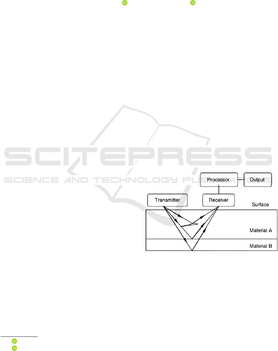
GPR Fig. 1 is broken down into the below subcate-

gories, which are categorized as geophysical surveys

and speciﬁcally involve the use of radar to probe the

surface of the ground. This method is very helpful

for locating items on the ground, especially utility

lines, where the gourd contains features like concrete,

metal, or plastic lines, cables and even masonry struc-

tures. GPR works by emitting high-frequency electro-

magnetic pulses into the earth’s surface and measur-

ing the reﬂection of the pulse that comes back from

the objects and interfaces lying in the ground. In this

study we use two methods to obtain object source im-

ages from GPR images: Hamiltonian Monte Carlo

and a U-net Neural Network.

https://orcid.org/0009-0009-7739-1832

https://orcid.org/0000-0002-3027-258X

Figure 1: GPR System.

1.2 Hamiltonian Monte Carlo

Markov Chain Monte Carlo (MCMC) methods are

widely used to obtain source images from GPR re-

sults. For instance (Hunziker et al., 2019) (Qin et al.,

2016) use Bayesian-based MCMC methods to sim-

ulate and reconstruct GPR source images. In this

work, we use a Hamiltonian Monte Carlo approach

(HMC) to do this task. HMC was initially devel-

oped in 1987 by (Duane et al., 1987) as a method

based on the idea of energy conservation and mini-

mal action path from Hamiltonian Mechanics (HM).

154

Khandelwal, J. and Pareek, D.

Enhancing Parameters Estimation in Subsurface Imaging with Ground Penetrating Radars.

DOI: 10.5220/0013263400004646

Paper published under CC license (CC BY-NC-ND 4.0)

In Proceedings of the 1st International Conference on Cognitive & Cloud Computing (IC3Com 2024), pages 154-160

ISBN: 978-989-758-739-9

Compared to standard random walk-in metropolis al-

gorithms, HM properties allow HMC methods better

convergence to the typical set-in problems with high

dimensionality. This is therefore very useful for GPR

problems where the solution space has the same di-

mensions as the number of pixels in the image (there-

fore for typical images of 64 × 64 pixels one has to

consider systems of dimensions up to 4096)

1.3 Neural Networks

The U-net ﬁg. 2 architecture, initially developed for

segmenting biomedical images, consists of two main

components: it contains an encoder and a decoder,

an encoder and a decoder. In semantic segmentation,

unlike in image classiﬁcation applications where the

main output is the primary goal, pixel-level accuracy

is needed, and a way to transfer the detected features

when they are processed at different encoder stages

back to the pixel domain is required (Ronneberger

et al., 2015). The encoder part of the U-net struc-

ture, depicted in Fig. 1, usually employs an exist-

ing classiﬁcation network like VGG or ResNet (He

et al., 2015). This component uses a layer of convo-

lution block made up of several numbers of convo-

lutions each of which is followed by down sampling

max pooling to extract multi-level features from the

input image. The decoder, which forms the second

half of the U-net, should be able to generate an out-

put map that is high in resolution and semantic con-

tent from a set of lower-resolution features obtained

by the encoder section. This process involves; up-

sampling operations on the feature maps; concatena-

tion of features; and more convolutional operations to

obtain per-pixel density maps.

2 METHODOLOGY

In this section, we explain our approach to solve the

GPR problem using HMC and Neural Network.

2.1 Selecting a Temp

To generate our GPR data we have used a forward

model simulation. The usual procedure for GPR im-

age reconstruction involves performing time evolu-

tion of a simulated source using Finite Time Dif-

ference Methods (FDTD) to simulate wave propaga-

tion for a candidate source distribution. Although

more efﬁcient approaches using other methods such

as Runge-Kutta schemes, (WAN, 2020) have been de-

veloped, these methods are often time-consuming and

resource-intensive. Therefore, in this study, we use a

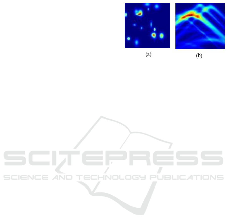
Figure 2: GPR image, (a) Forward model obtained from

Object Image (b) Object Image.

simpliﬁed method based on simple wave propagation

equations to build a forward model, that is, a simu-

lation of the resulting GPR image produced by a pro-

posed source. The resulting forward image will be

modelled by the equation (1).

A(r) = A

P(2∆t)e

−

2γr (1)

Where γ is a dampening constant depending on

the media properties, r is the Euclidean distance from

the GPR to each source and DT = r /u, where u is

the speed of light in the media, is the time taken to

travel from the GPR to the source. In the equation

above, the reader will recognize the typical equation

of an over-damped harmonic oscillator (hyperbolic

equations). This is the result of considering only the

evolution of the amplitude of the wave with time and

omitting all the imaginary terms that result in more

complicated interactions like destructive interference.

Other usual effects in this ﬁeld like refraction caused

by water droplets in the media have also been omitted

here and introduced in a simpliﬁed way in the source

model as Gaussian noise. The equation above can be

rewritten as propagator equation D = G · F where F

is the pixel-wise map of sources, G is the wave prop-

agator given by A(r) and D is the resulting image in

the GPR. We call the resulting image forward model

as shown in Fig 2 (a) and (b).

2.2 Hamiltonian Monte Carlo

Details of the Hamiltonian Monte Carlo method can

be found in (Betancourt, 2018). As usual, our Hamil-

tonian is the resulting sum of potential and kinetic

energy functions, where kinetic energy is indepen-

dent of spatial coordinates and potential energy is

independent of momentum coordinates 1. Momen-

tum values are generated pixel-wise with random nor-

mal distribution, with a standard deviation dependent

on the temperature of the system. The kinetic en-

ergy is then calculated as the classical kinetic energy

considering the identity as a mass matrix, therefore,

Enhancing Parameters Estimation in Subsurface Imaging with Ground Penetrating Radars

155

K(p

)

= 1/2pp2. The potential function is our ob-

jective function and it is through the gradient of the

potential that our state converges to the typical set.

The potential energy is calculated as the squared error

V (q) = 1/2(DGF)2 where D is the real forward im-

age, G is the propagator of the problem as described

above, and F is the current state of the HMC chain. At

each iteration, a new Hamiltonian resulting from new

kinetic and potential energies is calculated. The re-

sulting Hamiltonian evolves in time with the leapfrog

integration method.

For 0 ≤ n <

A ← A − E δV (q

)δq

n+1

← q

+ E p

← A

− 2δq(a

+ q)

End For.

Where T is the total time evolved and E is the

step size. This simple method allows us to evolve the

Hamiltonian in time following a path that minimizes

its action, as described by Hamilton equations. Note

that if K and V are scleronomic, Hamilton equations

reduce to

δK(p)

δp

(2)

d p

δV (q)

δq

(3)

Which bears similarity to the leapfrog algorithm.

The forward image used for the HMC method was

of size 64 × 64 and was generated using the forward

model described above for 1, 3 and 50 sources. The

simpliﬁed single-source scenario was used to build

and tune hyperparameters for the HMC model. Hy-

perparameters in HMC govern the evolution of the

state and its convergence to the typical set. These

parameters are typically referred to as Temperature

and step size, where the former governs the amount

of chaos or variation introduced to the system at each

iteration, and the latter is the step size used in the

leapfrog integrator to calculate the variation of the

Hamiltonian at each integration step. One of the difﬁ-

culties of the HMC method is to use optimal parame-

ters for convergence, which depend on the typical set

and the nature of the problem. In addition to the ones

described above, it is also useful to ﬁnd a good seed to

allow for faster convergence. To ﬁnd the best values

for these parameters (T, step size, seed) an exhaustive

search over common parameter ranges was conducted

in the iris-cluster (Varrette et al., 2014). After ﬁnd-

ing the best set of parameters, we run the HMC for

10,000 iterations for 1, 3 and 50 initial sources. To

compare the ﬁnal states to the initial simulation we

perform a structural similarity test on the ﬁnal states

smoothed with a Gaussian ﬁlter. For completeness,

we also compare the initial simulation and the ﬁnal

HMC state with a full waveform inversion model ob-

tained using back projection.

2.3 Neural Networks approach

As we see the in GPR data (see Fig. 2 & 3) every pixel

intensity deﬁnes the reﬂectivity and shows the object

property. It means we have to predict the exact values

of these pixels to ﬁnd the objects. Traditionally U-net

is used for segmentation and assigns class labels to

each pixel. But in our case, it is more of a regression

problem to predict the reﬂectivity values of pixels.

• Neural Networks Architecture: The network ar-

chitecture, inspired by U-net as illustrated in Fig.

1, consists of two main pathways: PATH A has

elements that compress, control or conﬁne: re-

gressive, directive and enclosed (left side of the

ﬁgure), PATH B has elements that open up, en-

courage, and set free: progressive, persuasive and

most encompassing (right side of the ﬁgure). The

compressive path is implemented with the general

architecture of a convolutional network. It suc-

cessively performs two convolutions of 3x3 with

the same padding and uses the ReLU activation

function; and then a max pooling of 2x2 with

a stride of 2 for down sampling. Thus, in the

down-sampling processes, the number of chan-

nels is doubled while the size of the feature maps

is reduced. Steps of the expansive path are up-

sampling the feature map, then followed by a con-

volution operation with a 2 x 2 ﬁlter, which is also

known as up-convolution that reduces the num-

ber of channels in the feature map by two at that

step. Which is then concatenated to a feature map

extracted from the compressive path at the same

level but with precise cropping. Two 3 x 3 con-

volutions and ReLU are next to each other, one

convolution is followed by ReLU. The cropping

is needed because the convolution operation crops

out a portion of the border in each instance of the

feature map. The network ends with a 1x1 convo-

lution layer at the last stage that transforms each

64-element vector into the output. Blue rectan-

gles denote the multi-channel feature maps. Next

to each rectangular ﬁgure, there is a number that

represents the number of channels; the x-y dimen-

sions are also provided in the lower left corner.

White rectangles are the duplicative feature maps

as indicated below. Some of the operations are

IC3Com 2024 - International Conference on Cognitive & Cloud Computing

156

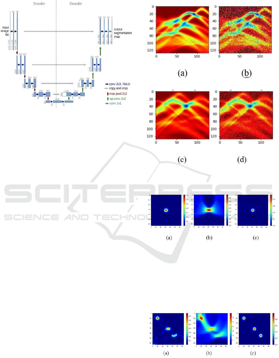
Figure 3: U-net architecture (example for 32x32 pixels in

the lowest resolution).

shown by the arrows linking these elements.

• Training: The input to the model is, image pairs

consisting of the input image and the object map

of the same image. Indeed we use stochastic gra-

dient descent for the training implementation. The

input images underlying our ﬁlters are of the di-

mension 128 x 128 pixels. For better detail cap-

turing, the batch size is selected to be 32 and the

learning rate is 1e-4. As for the loss function,

since our objective is less about trying to catego-

rize data as it is to predict it, we use Mean Squared

Error (MSE). It also enables this choice to make

the pixel intensities forecasts more accurate. To

effectively capture these intensity values, we im-

plement the ReLU function as our non-linear ac-

tivation. We have also added dropouts 0.4 to stop

overﬁt.

MSE = L

− y

)

(4)

• Data Augmentation: It is necessary to build an ap-

propriate level of invariance and robustness in the

network by applying the strategies of data aug-

mentation. We used the augmentations library for

this and added Gaussian noise to the data to make

it robust (Fig. 4).

3 RESULTS

In this section, we discuss our results from HMC and

Neural Network approach.

3.1 HMC

The ﬁnal state (object image) from the resulting HMC

chain is shown for 1, 3 and 50 sources in Fig. 5 to

Figure 4: Gaussian Noise Augmentation, (a) and (c) rep-

resent the Original image, (b) and (d) represent the Aug-

mented Image.

Figure 5: Left to right for 1 source, (a) Final state of the

HMC chain (b) source image obtained with backpropaga-

tion (c) real (simulated) source image

7 respectively. The resulting forward image of

the ﬁnal HMC state and the real image for the same

sources are shown in Figures 5 to 10. Table 1 shows

the values of SSI for all sources for both the HMC

result and backpropagation.

Figure 6: Left to right for 3 sources (a) Final state of the

HMC chain (b) source image obtained with backpropaga-

tion (c) real (simulated) source image

Enhancing Parameters Estimation in Subsurface Imaging with Ground Penetrating Radars

157

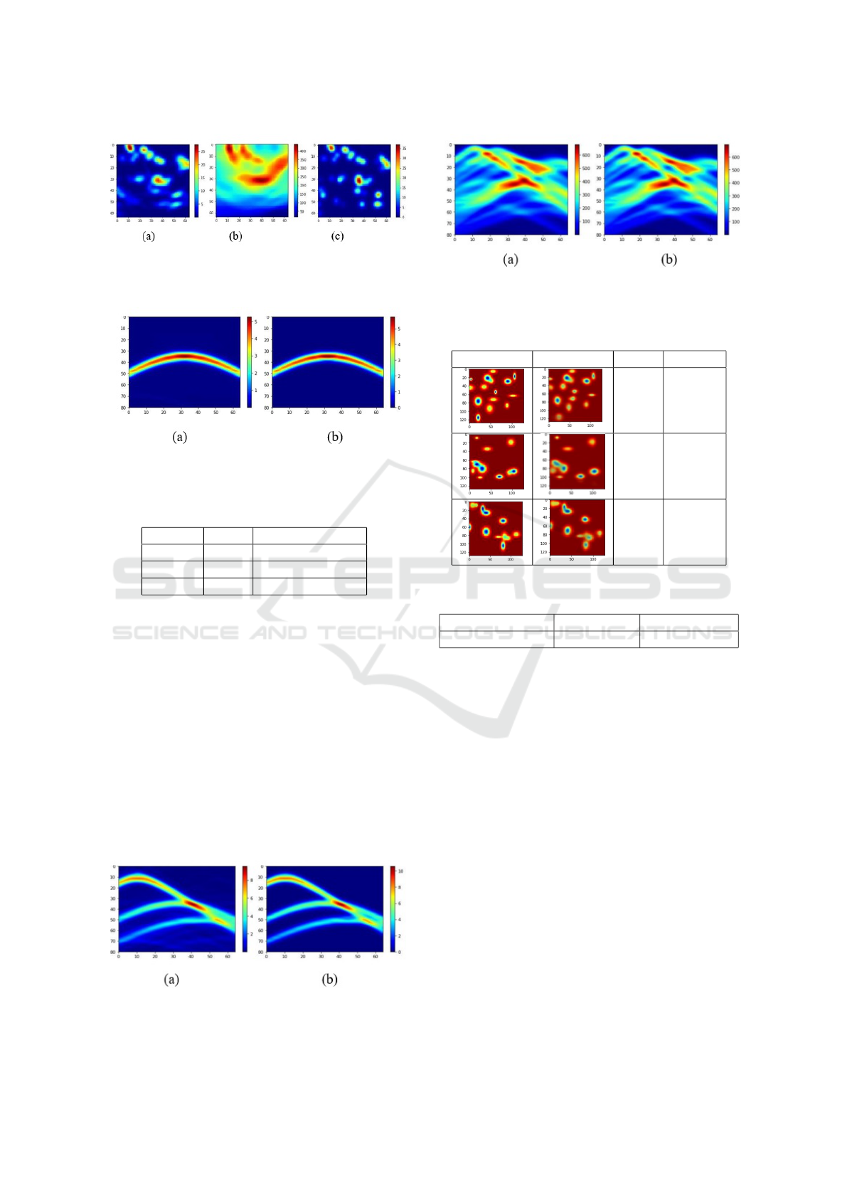
Figure 7: Left to right for 50 sources: (a) Final state of the

HMC chain (b) source image obtained with backpropaga-

tion (c) real (simulated) source image

Figure 8: From left to right for 1 source, (a) the forward

image of the HMC ﬁnal state and (b) the forward image of

the real source image

Table 1: SSI values for deferent numbers of sources.

Sources HMC Backpropagation

1 0.99 0.31

3 0.84 0.05

50 0.52 0.006

3.1.1 Neural Network

Table 2, shows the results from neural network pre-

dictions. We used the Multi-Scale Structural Simi-

larity Index (MSSIM) and Structural Similarity Index

(SSIM) to compare matrices (Higher values are bet-

ter). The table presents the mean values of the Multi-

Scale Structural Similarity Index (MSSIM) and Struc-

tural Similarity Index (SSIM) achieved by the U-net

model on the test data. These metrics quantify how

similar the U-net’s predicted object images are to the

ground truth images, with higher values indicating

better structural similarity and, consequently, better

performance.

Figure 9: From left to right for 3 sources: forward image of

the HMC ﬁnal state, forward image of the real source image

Figure 10: From left to right for 50 sources: forward image

of the HMC ﬁnal state, forward image of the real source

image

Table 2: Prediction result.

Label Prediction SSIM MSSIM

0.99 0.94

0.99 0.95

Table 3: Shows the mean values of SSIM and MSSIM on

test data.

Test data number Mean SSIM Mean MSSIM

1000 0.99 0.93

The purpose of Table 3, is two-fold: ﬁrst, it evalu-

ates the generalization performance of the trained U-

net model by reporting its mean SSIM and MSSIM

scores on a separate test dataset of 1000 samples. This

demonstrates the model’s ability to perform well on

unseen GPR data. Second, it provides a direct com-

parison point with the HMC results reported in Ta-

ble I, allowing the reader to appreciate the relative

strengths of the U-net approach, especially in scenar-

ios with many sources where the HMC method’s per-

formance declines.

Likewise, from the results presented in Table III

that demonstrate high mean SSIM and MSSIM on the

test data, conﬁdence can be gained with the proposed

U-net for subsurface imaging with GPR data. It sup-

ports the authors’ assertion that the U-net model is

more suitable for handling several sources of com-

plexity in the capturing of data than the HMC tech-

nique. In general, Table III is instrumental in measur-

ing the generalization capability of the U-net model

and provides valuable insight into this study; it un-

derscores the U-net model’s capacity to obtain highly

IC3Com 2024 - International Conference on Cognitive & Cloud Computing

158

accurate results in detecting subsurface sources in un-

seen data.

4 COMPUTATIONAL COST

ANALYSIS

However, besides the comparison of the performance,

the computational costs of the HMC and U-net should

be compared as well, since they play a critical role in

determining the feasibility of these approaches’ appli-

cation in practice.

4.1 Time Complexity

The Hamiltonian Monte Carlo (HMC) is an iterative

sampling tactic, and the time-consuming option in-

creases with the number of iterations needed to reach

convergence. Further, due to the high dimensions in-

duced by the number of pixels in the GPR image,

HMC’s time complexity becomes high. On the other

hand, the U-net neural network approach once trained

can predict in a single forward pass and hence the time

complexity will be constant irrespective of the input

size/complexity.

4.2 Resource Requirements

Dew Fletcher indeed pointed out that HMC is a com-

putationally dense method, especially for problems

with high dimensionality. Depending on the size of

the objective function and the number of parameters

there can be a high computational cost, computations

of the objective function and its gradients are needed

in each iteration which may be expensive and can re-

quire parallel computing resources or special purpose

hardware acceleration.

On the other hand, the U-net model even though

it may be time-consuming during training, can take

advantage of the parallelism that modern GPU offers

for inference. The evaluation of the model shows that

it can construct a prediction system based on the new

data with relatively low overhead helping to reduce

the computational load and increase the efﬁciency of

the solution for deployment.

4.3 Practical Implications

Therefore, near real-time predictions are mandatory,

such as in real-life applications of GPR, the constant

time complexity and the insigniﬁcant inference over-

head of the U-net model seem to be concomitantly

beneﬁcial. Also, it is crucial to note that the actual-

ization of the model requires ﬂexibility in the choice

of deployment mechanism.When the trained U-net

model is concluded on resource limited devices or

edge computing platforms, it makes the model very

suitable for use.

However, for situations where the distinction be-

tween different categories is important or the results

need to be presented and analyzed statistically the

HMC method may seem preferable. Covariance and

the ability to follow the Markov Chain means that the

changes in each pixel and the statistical properties in

the image such as the value distribution can be ana-

lyzed and this could prove useful in research and anal-

ysis oriented applications.

However, it is necessary to emphasize that when

choosing between computational cost and accuracy,

one should think more about the special conditions

of the particular application. In cases where there is

ample computation to be done and where exact so-

lutions are desired the HMC method could be used

though it has been mentioned to be computationally

more expensive. On the other hand, where informa-

tion is in limited supply or time is critical and near

real time predictions are necessary then perhaps the

U-net model despite having slightly less interpretabil-

ity may be more beneﬁcial.

5 CONCLUSION

It can be observed that the usage of U-net NN has

enhanced the results as compared to HMC. This im-

provement however is not without a downside since

Unet requires a large amount of data to train the model

and HMC does not. HMC also enables tracking

the changes in each single pixel through the Markov

Chain thus enabling statistical calculation such as

variance and value distribution for each single pixel,

which Unet does not enable because it was unde-

ﬁned. Further investigations might attempt to use a

hybrid method combining both techniques, as well

as a more complex forward model with interactions

between wavefronts and more dispersion effects with

the underground media.

REFERENCES

(2020). An interpolating scaling functions method with

low-storage ﬁve-stage fourth-order explicit runge-

kutta schemes for 3d ground penetrating radar simula-

tion. Journal of Applied Geophysics, 180:104128.

Betancourt, M. (2018). A conceptual introduction to hamil-

tonian monte carlo.

Duane, S., Kennedy, A., Pendleton, B. J., and Roweth,

Enhancing Parameters Estimation in Subsurface Imaging with Ground Penetrating Radars

159

D. (1987). Hybrid monte carlo. Physics Letters B,

195(2):216–222.

He, K., Zhang, X., Ren, S., and Sun, J. (2015). Deep resid-

ual learning for image recognition.

Hunziker, J., Laloy, E., and Linde, N. (2019). Bayesian full-

waveform tomography with application to crosshole

ground penetrating radar data. Geophysical Journal

International, 218(2):913–931.

Qin, H., Xie, X., Vrugt, J. A., Zeng, K., and Hong, G.

(2016). Underground structure defect detection and

reconstruction using crosshole gpr and bayesian wave-

form inversion. Automation in Construction, 68:156–

169.

Ronneberger, O., Fischer, P., and Brox, T. (2015). U-net:

Convolutional networks for biomedical image seg-

mentation. arXiv e-prints, page arXiv:1505.04597.

Varrette, S., Bouvry, P., Cartiaux, H., and Georgatos, F.

(2014). Management of an academic hpc cluster: The

ul experience. In 2014 International Conference on

High Performance Computing Simulation (HPCS),

pages 959–967.

IC3Com 2024 - International Conference on Cognitive & Cloud Computing

160