Atmospheric Correction of Sentinel-2 Images Using Deep Learning
Stavan Shah
1 a
, Kahaan Patel
1 b
, Ankur Garg
2 c
and Shivangi Surati
1 d
1
Computer Science and Engineering, School of Technology, Pandit Deendayal Energy University, Gandhinagar, Gujarat,
India
2
Indian Space Research Organization, Ahmedabad, Gujarat, India
Keywords:
Atmospheric Correction, Pix2Pix, Conditional Generative Adversarial Network, Remote Sensing, Deep
Learning, Sentinel-2
Abstract:
Remote sensing relies heavily on pre-processing steps, one of which is the Atmospheric Correction (AC).
It corrects the effects of atmosphere on satellite images. This makes it a vital step in ensuring accurate es-
timation of land Surface Reflectance (SR) that can be used in various downstream applications. But such
conventional AC methods are computationally expensive because they use physics-based radiative transfer
codes, need metadata from each image as well as many different atmospheric parameters which might not
all be easy to estimate accurately. A novel Deep Learning (DL) model designed for AC without having to
explicitly estimate atmospheric parameters is proposed in this research. The deep learning model was trained
using a wide-ranging dataset collected by Google Earth Engine that included four bands of Sentinel 2 images
covering all states in India. The proposed approach directly predicts SR values from Sentinel-2 satellite im-
agery using this data driven method. It generated promising results by accurately estimating SR values with
ground measurements and sentinel input data experiments confirming this point too. This approach not only
simplifies the AC process but also achieves comparable or even superior performance compared to traditional
physics-based methods. The evaluation results show that Pix2Pix model has good performance, with average
SSIM, PSNR, RMSE and MAE of 0.96, 42.14, 0.0097 and 0.0071 respectively. The experimental findings
underscore the potential of deep learning as a robust and efficient alternative for atmospheric correction in
remote sensing applications.
1 INTRODUCTION
Through remote sensing, the images taken from
above the earth’s surface are essential for mon-
itoring and understanding. Unfortunately, these
images are normally tainted with atmospheric ef-
fects such as scattering and absorption that can dis-
tort actual surface reflectance. Atmospheric cor-
rection is a critical pre-processing step in remote
sensing that aims at removing these atmospheric
influences to give precise values of surface re-
flectance (Zhu and Xia, 2023), (Zhang et al., 2022).
The main objective of AC is to transform Top-
Of-Atmosphere (TOA) reflectances into Bottom-Of-
Atmosphere (BOA)/surface reflectances. This en-
ables interpretation and investigation of remote sens-
a
https://orcid.org/0009-0000-1778-1745
b
https://orcid.org/0009-0005-9981-6257
c
https://orcid.org/0000-0002-2872-5690
d
https://orcid.org/0000-0003-4381-5130
ing data more accurately. Complex mathematical for-
mulation involving the aerosol content, Rayleigh scat-
tering as well as water vapor among others are neces-
sary to convert TOA Reflectance to SR. An example
includes 6S (Second Simulation of the Satellite Signal
in the Solar Spectrum) model that is used to approx-
imate atmospheric parameters depending on radiative
transfer principles (Ilori and Knudby, 2020). Parti-
cles such as atmospheric gases, aerosols and others
scatter and absorb sunlight and hence, the process of
atmospheric correction is extremely important for any
satellite imagery analysis.
The Sentinel-2 mission is outstanding among the
numerous Earth observation satellites due to its ex-
tensive coverage and high resolution. It belongs to
Copernicus program of European Space Agency and
offers multispectral imagery with 13 spectral bands
across visible, near infrared and short wavelength in-
frared parts of electromagnetic spectrum. These are
useful in land cover characterization, vegetation in-
dices retrieval and water quality monitoring thus mak-
Shah, S., Patel, K., Garg, A. and Surati, S.
Atmospheric Correction of Sentinel-2 Images Using Deep Learning.
DOI: 10.5220/0013303900004646
Paper published under CC license (CC BY-NC-ND 4.0)
In Proceedings of the 1st International Conference on Cognitive & Cloud Computing (IC3Com 2024), pages 175-185
ISBN: 978-989-758-739-9
Proceedings Copyright © 2025 by SCITEPRESS – Science and Technology Publications, Lda.
175

ing the Sentinel-2 data paramount in various envi-
ronmental and agriculture applications (Phiri et al.,
2020).
These methods are usually based on physics
which require extensive computational resources and
accurate knowledge of the atmosphere variables (Liu
et al., 2022). In the recent years Pix2Pix model,
a GAN variant, has achieved impressive results in
image-to-image translation tasks. In the proposed
work, while trained on large paired datasets of TOA
and SR images for instance, Pix2Pix models gener-
ate high-quality SR images directly from TOA in-
puts by learning their complex mapping. The other
advantages of using this model is flexibility, direct
optimization through end-to-end learning framework,
generalization competencies and robustness to devia-
tions in input data and high quality outputs. The gen-
erated images are then compared using several eval-
uation parameters such as Structural Similarity Index
Measure (SSIM), Peak Signal to Noise Ratio (PSNR),
Root Mean Square Error (RMSE), and Mean Abso-
lute Error (MAE) with their ground truths.
The organization of the paper is as follows. The
detailed discussion of prior methods and techniques
of atmospheric correction is presented in Section 2.
The data, model architecture and evaluation tech-
niques incorporated in this work are presented in Sec-
tion 3. The evaluated results of the proposed method-
ology are presented and discussed in section 4. Sec-
tion 5 wraps up by summarising the main conclusions
and going over the probable next lines of research.
2 RELATED WORK
Several algorithms for Aerosol Optical Depth (AOD)
retrieval from TOA data have been developed and
are widely used. Some of these algorithms are Dark
Target (Remer et al., 2020), Deep Blue (Hsu et al.,
2013) and Multi-Angle Implementation of Atmo-
spheric Correction (MAIAC). However, one of the
main issues in AOD retrieval is the difficulty in accu-
rately parameterizing the basic aerosol optical proper-
ties which leads to large uncertainties. Additionally,
there exist other methods used for Columnar Water
Vapor (CWV) estimation. Some common approaches
include Low-Rank Subspace Projection-Based Wa-
ter Estimator (LRP-WAVE) (Acito and Diani, 2018)
and Atmospheric Pre-corrected Differential Absorp-
tion (APDA) (Schl
¨
apfer et al., 1998). Neverthe-
less, these algorithms suffer from drawbacks such
as being based on physical assumptions or requiring
hard-to-get parameters respectively. SR uncertainty
comes from two factors; AOD and CWV estimated er-
rors during SR derivation from TOA data estimation,
AODs alone should not be a priority compared to both
because their accuracies affect each other’s accuracy
too much and hence, they need accurate estimates.
On the flip side, image-based methods achieve AC
solely through the use of images taken from satellite
or aerial sensors; they don’t need any atmospheric pa-
rameters as input but instead utilize only the infor-
mation inherent in the image itself. The Dark Ob-
ject Subtraction is one of the most basic techniques in
which at least two targets with low and high reflec-
tivity from within scene must be identified. Another
image-based AC model called Quick Atmospheric
Correction (QuAC) (Bernstein et al., 2012) works on
a different assumption- average group material spec-
tra remains same across various scenes. If there are
more than ten different things present in background
then QuAC performs well. Although they are in-
tuitive and computationally efficient, these methods
lack ability to quickly estimate surface reflectance
values at first order due to their accuracy under con-
ditions involving seasonal and spectral variation.
Based on deep learning model approaches, two
atmospheric correction deep learning models were
trained and evaluated using one hundred thousand
batches of 40 transformed reflectance spectra to radi-
ance by means of MODTRAN (Basener and Basener,
2023). It allowed the deep learning model to fig-
ure out the physics of radiation transfer from MOD-
TRAN. For this purpose, they compared two meth-
ods to estimate corrections in a well-known QuAC
model which is based on constant mean endmem-
ber reflectance assumption. Using the HY-1C CZI as
a case study, a new approach is presented in (Zhao
et al., 2023) to atmospheric correction based on deep
learning (SSACNet). The third dimension convolu-
tion was applied to extract spatial and spectral fea-
tures for the image while second dimension convolu-
tion was investigated for recovery of lost spatial in-
formation. According to in-situ data, the SSACNet
shows decent performance having average correlation
coefficient of 0.89 and Absolute Percentage Deviation
(APD) ranging from 21.53% to 35.41% in four bands.
To do AC, all deep learning models that could
match the efficiency and accuracy of physics-based
techniques in computing are observed. Additionally,
DL models do not need any climatic or geometric
parameters as input. Compared to those based on
physics, computational power usage is reduced with
DL models. This is because, they can learn features
automatically and thus, making it easy to build and
train models. Stacked autoencoders, Convolutional
Neural Networks (CNNs) (Wang et al., 2022), and vi-
sion transformers (Liu et al., 2024) are some promis-
IC3Com 2024 - International Conference on Cognitive & Cloud Computing
176

ing methods used in remote sensing imaging appli-
cations such as spectral spatial and temporal feature
extraction being performed by them.
In the proposed work, a new method is described
that uses DL for atmospheric correction in remote
sensing data without the need for atmospheric param-
eters and geometric parameters; only input images are
considered. To the best of our knowledge, the pro-
posed methodology is the first approach that utilizes
Pix2Pix model for AC. The deep learning Pix2Pix
model was developed using a large dataset from dif-
ferent states of India in order to improve its perfor-
mance and generalization.
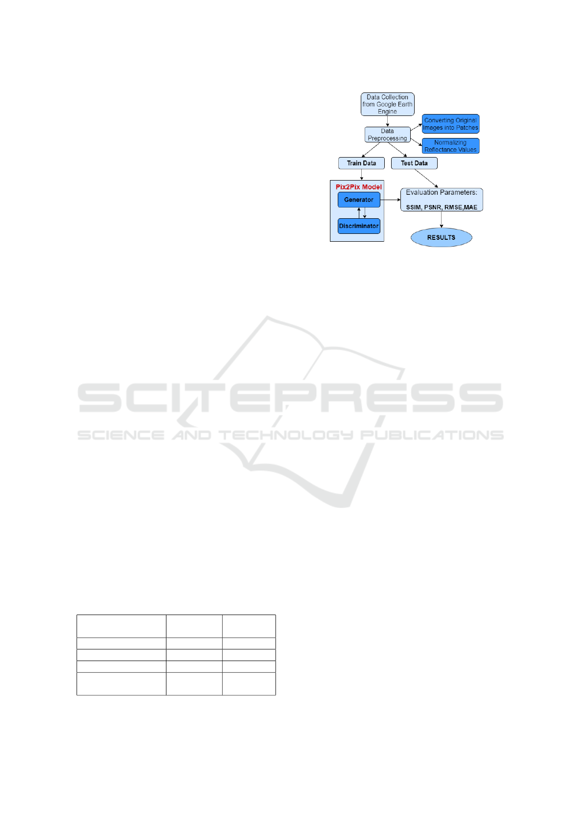
3 PROPOSED METHODOLOGY
The flowchart presented in Figure 1 outlines the steps
of proposed methodology for atmospheric correction
of sentinel-2 images.
3.1 Dataset Collection
The proposed research used data from Google Earth
Engine, a cloud-based platform that provides access
to a wide range of geographical datasets and satellite
images. Both atmospherically corrected and incor-
rected satellite images were gathered for this study.
Atmospherically incorrected images are TOA mea-
surements taken by satellite sensors without compen-
sating for scattering or absorption by atmosphere. At-
mospherically corrected pictures have been processed
to eliminate atmospheric interference so that surface
reflectance values accurately represent features on
earth’s surface.
In this study, Sentinel-2 satellite data from the
Google Earth Engine is used. Sentinel-2 is a Euro-
pean Space Agency (ESA) satellite mission designed
for monitoring Earth’s land and coastal areas. The
usual number of spectral bands in Sentinel 2A/B MSI
imagery is 13 bands. However, only four specific
bands having 10m resolution were included in this
study as shown in Table 1.
Table 1: Sentinel-2 Band Information.
Band Wavelength
(nm)
Resolution
(m)
Band 2 (Blue) (b) 490 10
Band 3 (Green) (g) 560 10
Band 4 (Red) (r) 665 10
Band 8 (Near-
Infrared) (vnir)
842 10
Figure 1: Model flowchart.
A total of 1000 images were collected. Each im-
age is atmospherically incorrected and its respective
atmospherically corrected image mapped together in
order to perform image to image translation. The im-
ages cover various regions across India, providing a
diverse and representative sample for analysis. There
are two ways to visualize the data:
1. True color composite: In true color composite im-
agery, the red, green, and blue bands (Bands 4,
3, and 2 respectively) are combined to replicate
human vision, producing an image akin to what
the human eye perceives. RGB images (true color
composite) are visualized in Figure 2a, where
(1), (3) are Atmospherically Incorrected Images
whereas (2), (4) are their Atmospherically Cor-
rected Images respectively.
2. False color composite: False color composite uti-
lizes non-visible bands, typically near-infrared
(Band 8), red (Band 4), and green (Band 3), to
highlight features not discernible to the human
eye. This composite reveals vegetation health,
land-water boundaries, and other environmental
characteristics, enhancing analysis in applications
such as agriculture, forestry, and environmental
monitoring. The False color images composite of
2 sample data are visualized in Figure 2b, where
(1) and (3) are Atmospherically Incorrected Im-
ages whereas (2) and (4) are their Atmospheri-
cally Corrected Images respectively.
3.2 Data Preprocessing
After gathering data from Google Earth Engine, orig-
inal dataset consisted of images in different sizes like
1000x1000 and 1200x1200 pixels. These patches
were taken out from input (atmospherically incor-
rected) and ground truth (atmospherically corrected)
images both at 256x256 pixels to standardize input
Atmospheric Correction of Sentinel-2 Images Using Deep Learning
177

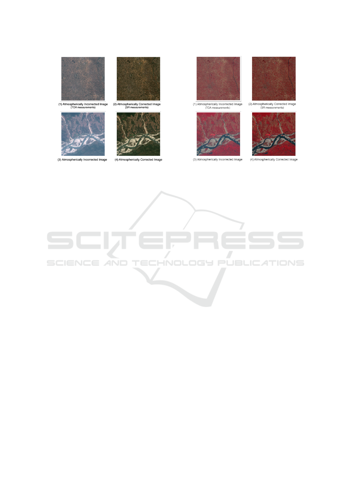
(a) True color composites. (b) False color composites.
Figure 2: Comparison of true and false color composites.
data for further analysis and processing. Hence, each
image irrespective of its original dimensions became
(256, 256, 4) where ’4’ refers to four bands denoting
red, green, blue and near-infrared channels. In addi-
tion, top of atmosphere and surface reflectance mea-
surements obtained through satellite imagery usually
range between 0-30000.
Each measurement was divided by 10000 as an
important preprocessing step because this normaliza-
tion process has several benefits such as scaling pixel
values into standard range so that they can be con-
sistently compared across different images; secondly
during training ML algorithms tend to work more sta-
ble and converge faster when their pixel values are
normalized over smaller ranges. Moreover, the col-
lected dataset was split into two sets: training set and
testing set. Among 1000 images, 800 were employed
for model training while remaining 200 served as test
data.
3.3 Model Architecture
In the field of transforming pictures into other pic-
tures, Pix2Pix model is a very important and use-
ful tool. It provides a strong method for con-
verting input images to desired outputs which sup-
ports different applications like image denoising,
style transfer or semantic segmentation. For satel-
lite imagery atmospheric correction, this model can
be used to convert atmospherically incorrected im-
ages (rep-resenting top of atmosphere measurements)
into atmospherically corrected (depicting surface re-
flectance measurements) that is vital for improving
the quality and accuracy of satellite image analysis.
The structure of the Pix2Pix model includes two ma-
jor parts as discussed.
3.3.1 Generator
The generator usually takes as input the images
with incorrect atmosphere corrections (TOA measure-
ments), which are typically represented as tensors of
shape (256, 256, 4) as shown in Figure 3. The role of
the generator is to convert input images (atmospheri-
cally incorrected images representing TOA measure-
ments) into desired outputs (atmospheric corrected
images representing SR measurements). The archi-
tecture of this generator is designed such that it can
collect and elaborate upon spatial as well as spectral
characteristics present in input images while deliver-
ing accurate results that are visually pleasing. Struc-
ture of a generator involves downsampling and up-
sampling parts for extracting abstract features from
input images and generating output ones correspond-
ingly (Figure 3). In Pix2Pix model’s generator, an al-
tered version U-Net architecture was used that is effi-
cient and widely adopted in neural network design for
image-to-image translation tasks. This alteration in-
cludes encoder-decoder framework with skip connec-
tions enabling both down-sampling and up-sampling
operations while keeping intact spatial information
preservation capabilities within them.
Generator has two main layers:
1. Encoder: The encoder of the Pix2Pix model is
composed of various blocks where each block
contains a convolutional layer, batch normaliza-
tion and Leaky ReLU activation function. This
arrangement enables the encoder to extract high-
level features from input images effectively as
it reduces their spatial dimensions progressively.
IC3Com 2024 - International Conference on Cognitive & Cloud Computing
178

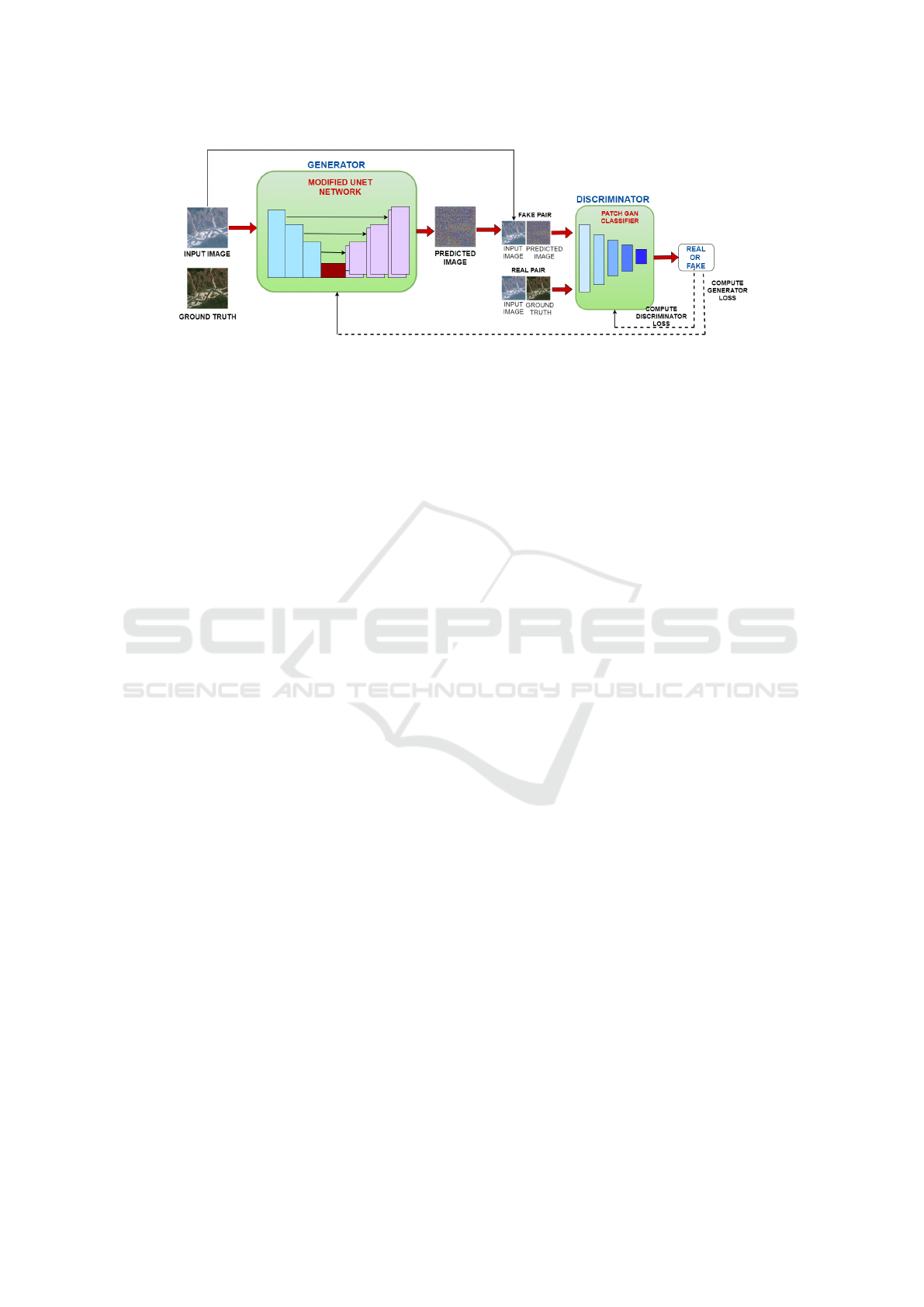
Figure 3: Pix2Pix architecture.
Each layer in this part consists of:
• Convolutional Layer: Every block begins with
a convolutional layer that applies a set of learn-
able filters to the input feature. These fil-
ters are designed to capture spatial information
and local patterns present in input images, thus
promoting feature extraction and representation
learning.
• Batch Normalization: The activations for each
layer across the mini-batch are stabilized by ap-
plying batch normalization after the convolu-
tional layer.
• Leaky ReLU Activation: After batch normal-
ization, applying a Leaky ReLU activation
function brings non-linearity into model that
helps it capturing complex features. It al-
lows small gradients for negative i/p values that
avoids vanishing gradient problem while pro-
moting more stable effective learning.
2. Decoder: The decoder of the Pix2Pix model is
made up of a series of blocks that mirror the en-
coder, which itself consists of transposed con-
volutional layers along with batch normalization,
dropout (used in the first 3 blocks), and ReLU ac-
tivation. This also includes skip connections be-
tween corresponding encoder and decoder blocks
to allow information to move through the system
more easily while retaining spatial details. Each
decoder layer has:
• Transposed Convolutional Layer: Each block
in the decoder begins with a transposed con-
volutional layer, or deconvolution/upsampling
layer. It enlarges input feature maps so that
higher resolution output images can be recon-
structed by the decoder.
• Batch Normalization: Activations are stabi-
lized and training is speed up by applying
batch normalization after the transposed convo-
lutional layer.
• Dropout (Applied to the First 3 Blocks): Over-
fitting is prevented and generalizability en-
hanced by applying dropout to first three blocks
in the decoder.
• ReLU Activation: Non-linearity is brought
about and feature representation heightened
following batch normalization through an ap-
plication of ReLU activation function. Sparse
passing of only positive values to next layer(s)
promoted by ReLU.
Allowing the model to retain and propagate important
spatial information throughout the network, skip con-
nections between encoder and decoder blocks (as pic-
tured in Figure 4) help in generating output images
with fine-grained details during reconstruction. In
fact the shown design of U-Net like this one also guar-
antees that during image-to-image translation process
by Pix2Pix; spatial features are captured or preserved
effectively at all levels of resolution.
The architecture of generator model is shown in
Figure 4, where first half acts as an encoder which
downsamples input image size while second part acts
as a decoder which upsamples it back again with skip
connections between them.
3.3.2 Discriminator
In the Pix2Pix conditional generative adversarial net-
work, a discriminator acts as a convolutional Patch-
GAN classifier, which means that it is designed to tell
apart real image patches from fake ones. During ad-
versarial training, it provides the generator with feed-
back about how well it creates natural-looking im-
ages. Every block in the discriminator performs a se-
quence of operations (Figure 5): Convolution, Batch
Normalization, Zero Padding (in some layers), Leaky
ReLU activation. This design allows the discrimina-
tor to extract features from image patches and learn
discriminative representations for classification. Af-
ter the last layer of the discriminator, there is an out-
put shaped as follows: (batch-size, 30, 30, 1). In this
Atmospheric Correction of Sentinel-2 Images Using Deep Learning
179

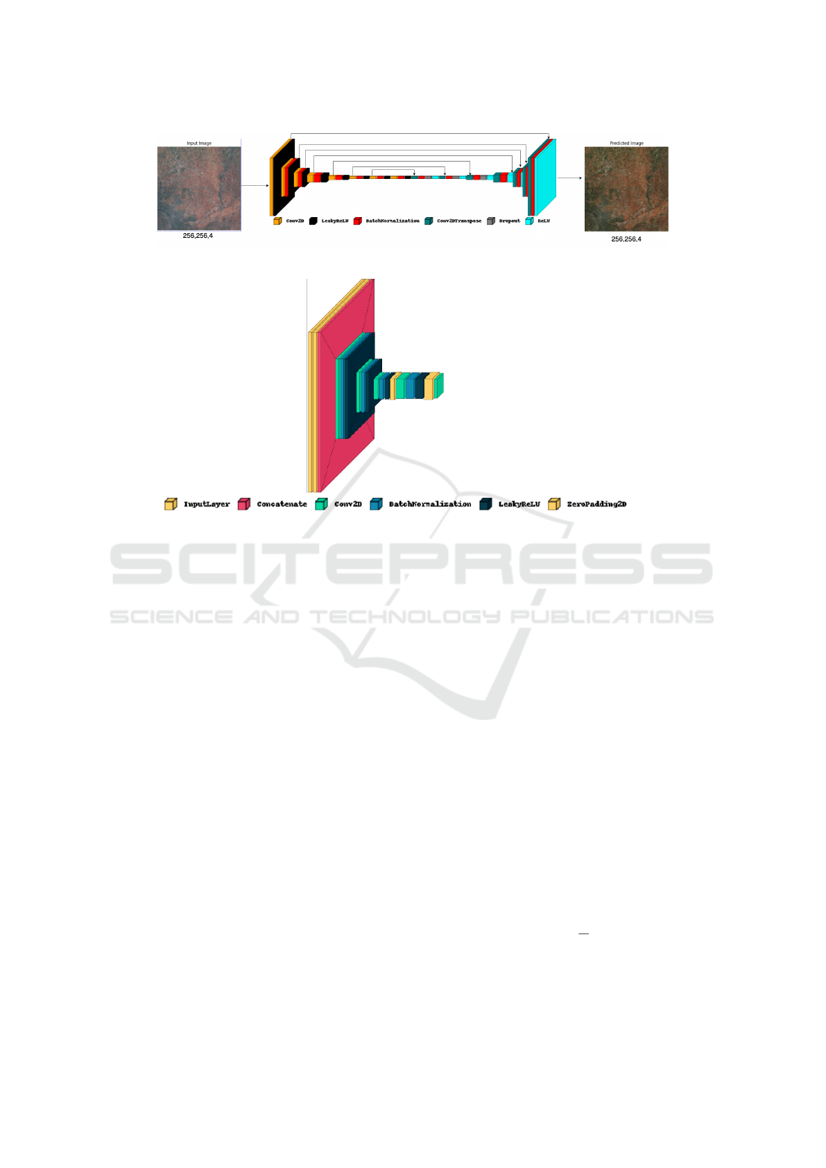
Figure 4: Generator architecture.
Figure 5: Discriminator architecture.
case, each 30 x 30 image patch classifies a 70 x 70
section of the in-put image. Such patch-wise classi-
fication strategy lets the discriminator concentrate on
local image details instead of global ones, thus mak-
ing it more effective for image-to-image translation
tasks. The discriminator receives two inputs as shown
in Figure 3:
1. Real Pair: Input image (atmospherically incor-
rected image) and target image (atmospherically
corrected image), which should be classified real
by discriminator.
2. Fake Pair: The input image (atmospherically in-
corrected image) and the generated image (image
generated by generator), which should be classi-
fied as fake by it.
In order to process these inputs, they are concate-
nated along channel axis using tf.concat([inp, tar],
axis= -1) so that a composite input containing both
input images as well as corresponding ground truth
images/generated images can be created.
By making use of this joint input, discriminator
becomes able to distinguish between real and fake
pairs of images thereby giving adversarial feedback to
generator which in turn helps it produce more believ-
able output pictures. Through this back-and-forth be-
tween generator and discriminator components within
Pix2Pix model itself learns how make good trans-
lations among different types of pictures while at
same time ensuring that all atmospherically wrong-
looking inputs get transformed into atmospherically
right ones. Discriminator architecture is presented in
Figure 5 below where first two layers represent in-
put images being concatenated in second layer (pink
layer). Various operations performed on concatenated
pair are depicted in Figure 5.
3.4 Model Training
The training steps can be divided into several impor-
tant parts which serve to improve the robustness as
well as accuracy of deep learning models.
1. Loss Functions: In Pix2Pix, the generator loss
involves multiple components that are useful for
guiding the training process. These components
are such as:
• L1 Loss: This measures the difference between
pixels in generated images and those in orig-
inal images also called Mean Absolute Error
(MAE) loss.
L1 Loss =
1
N
N
∑
i=1
|G(x
i
) − y
i
| (1)
• Generator GAN Loss: It is derived through
an adversarial training process based on dis-
criminator output which measures how good or
IC3Com 2024 - International Conference on Cognitive & Cloud Computing
180

bad our generated samples are when compared
against real ones.
L
G
= −E
z
[log(D(G(z)))] (2)
• Generator Total Loss: This is aggregate of L1
loss with a weighted generator GAN loss. Goal
is to balance image fidelity and image realism
during training.
Gen Total Loss = L1 Loss +λ · Gen GAN Loss
(3)
• Discriminator Loss: The discriminator loss
function measures the discrepancy between the
discriminator’s predictions (probability scores)
and the ground truth labels (real or fake).
Discriminator Loss = -
1
N
N
∑
i=1
[y
i
log(D(x
i
))+
(1 − y
i
)log(1 − D(x
i
))] (4)
2. Optimization Algorithm: The Adam optimizer
was used to train our deep learning model with
a learning rate of 0.0002. It ensures fast con-
vergence and optimization by gradient descent.
Adam’s adaptive learning rate mechanism that ad-
justs based on the first and second moments of
the gradients, provides a balance between con-
vergence speed and stability, crucial for the ad-
versarial nature of GANs. This adaptability helps
in achieving faster convergence and handling the
complex, non-linear transformations required for
atmospheric correction, where pixel-wise accu-
racy is critical. Momentum in Adam further
smooths the optimization path, leading to more
stable and reliable training outcomes. A learn-
ing rate of 0.0002 has been empirically validated
across various implementations of GANs, includ-
ing Pix2Pix, ensuring high quality image gener-
ation. This effectively balances need for quick
convergence without sacrificing stability, avoid-
ing the pitfalls of divergence seen with higher
rates and the slow training of lower rates. The
robustness of Adam to noisy gradients, a common
challenge in GAN training, enhances its suitabil-
ity for atmospheric correction, ensuring consis-
tent and accurate correction across diverse atmo-
spheric conditions and geographical regions.
3. Batch Processing and Summary: Mini-batch
stochastic gradient descent was applied through-
out training, using a batch size of 2. This ap-
proach helps save memory space while speeding
up the training process. The model parameters
are updated based on small subsets of the train-
ing data. Furthermore, a summary after every 10
epochs is created that include model predictions
on three randomly selected images from dataset
using checkpointed model at that epoch. At these
checkpoints, both the Generator and Discrimina-
tor models were saved to preserve their progress
in training.
4. Epochs and Early Stopping: Training lasted for
100 epochs (equivalent to 80,000 steps) but had an
early stopping criterion based on validation loss
to avoid overfitting network weights. With early
stopping, one can monitor how well the model
performs during training and stop when there is
no improvement in validation performance.
3.5 Evaluation Parameters
Evaluating model performance is crucial to assess the
fidelity and accuracy of the generated images com-
pared to ground truth images (atmospherically cor-
rected). Ground truth images provide a reference for
the desired output, allowing us to quantitatively mea-
sure the similarity between the generated/predicted
images and the true images. The evaluation param-
eters used for assessing the performance of Pix2Pix
model on both the training and testing datasets in-
clude:
1. Structural Similarity Index (SSIM): It measures
similarity between two images based on their lu-
minance, contrast and structure where difference
in perception between generated and ground truth
images is measured.
2. Peak Signal-to-Noise Ratio (PSNR): PSNR mea-
sures the ratio between the maximum possible
power of a signal and the power of corrupting
noise that affects the fidelity of its representation.
It quantifies the quality of the generated images
compared to the ground truth images.
3. Root Mean Squared Error (RMSE): RMSE mea-
sures the average difference between values pre-
dicted by the model and the observed values. It
represents square root of average of the squared
differences between predicted and observed val-
ues.
4. Mean Absolute Error (MAE): MAE measures the
average absolute difference between the predicted
and observed values. It provides a more intuitive
understanding of the average error magnitude.
Atmospheric Correction of Sentinel-2 Images Using Deep Learning
181

4 RESULTS
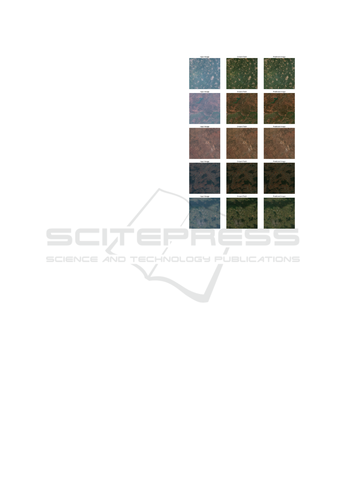
4.1 Predicting Images on Test Set
The model performed well on the test dataset, produc-
ing atmospherically corrected images that were very
similar to the corresponding ground truth images. The
synthesized image showed features and visual appear-
ances in common with the truth image. It reproduced
such things as texture, color tones and structural com-
ponents correctly which shows that it can capture de-
tailed patterns properly. Such similarity is shown in
Figure 6 where predicted (generated) images are com-
pared against their respective input images and in-
putted ground truths.
4.2 Evaluation Metrics
SSIM, PSNR, RMSE and MAE are used for evaluat-
ing quality of generated images compared to ground
truth images in image processing tasks. Range of
SSIM values is from -1 to 1, where 1 indicates per-
fect similarity between the images. Good SSIM val-
ues typically range between 0.9 and 1, indicating high
similarity and good quality. SSIM values below 0.5
are generally considered poor and may indicate sig-
nificant differences between the images. PSNR val-
ues are expressed in decibels (dB). Higher PSNR val-
ues indicate better quality, with values closer to infin-
ity representing perfect reconstruction. PSNR values
above 30 dB are typically considered good for most
applications. PSNR values below 20 dB may indicate
significant distortion and poor quality. If the values
of both RMSE and MAE are decreasing then it can
be considered that difference in pixels of ground truth
and generated images is reduced and both the images
are getting more similar to each other.
The below tables (Tables 2 and 3) depicts the min-
imum, maximum, mean and standard deviation of
all evaluation parameters. Values in Table 2 are the
evaluation parameters that are recorded before train-
ing process and in that the images are only gener-
ated via Pix2Pix generator model (similar to U-net).
Whereas, values in Table 3 are the evaluation param-
eters that are recorded after 100 epochs of training
the Pix2Pix model. There is a significant change
in values between these tables. Starting with SSIM,
which assesses the similarity between two images, a
mean SSIM value of -0.0025 with a standard devia-
tion of 0.0605 is shown in Table 2. This indicates poor
matching between the generated and ground truth im-
ages before training. In contrast, a significant im-
provement in SSIM metrics is revealed in Table 3,
with a mean value of 0.961 and a standard deviation
Figure 6: Generated images.
of 0.068. This substantial enhancement demonstrates
the model’s ability to produce images that closely
resemble the ground truth after training. 95% of
SSIM values are greater than 0.85 which indicates
that model is efficiently generating images similar to
ground truth. SSIM values recorded for test dataset
are described in Figure 7a.
Moving on to PSNR, Table 2 demonstrates a mean
PSNR value of 11.0188 dB with a standard deviation
of 0.6115 dB. These values indicate low image qual-
ity before training, as higher PSNR values correspond
to better image fidelity. How-ever, Table 3 shows a re-
markable improvement in PSNR metrics, with a mean
value of 42.14 dB and a standard deviation of 5.51 dB.
The drastic increase in PSNR reflects a significant en-
hancement in image quality after training, suggesting
that the model produces images with reduced noise
and improved fidelity. 97.5% of PSNR values are
greater than 30 that indicates that model is efficiently
generating images similar to ground truth. The PSNR
values recorded for test dataset are described in Fig-
ure 7b.
Next, Table 2 exhibits mean RMSE and MAE
values of 0.281 and 0.219, respectively, with stan-
dard deviations of 0.021 and 0.017. These values
indicate relatively high errors between generated and
IC3Com 2024 - International Conference on Cognitive & Cloud Computing
182

Table 2: Evaluation metrics before training.
Evaluation Parameters Maximum value Minimum value Mean value Standard Deviation
SSIM 0.00202 -0.0336 -0.0025 0.0605
PSNR 12.663 7.0231 11.0188 0.6115
RMSE 0.445 0.232 0.281 0.021
MAE 0.345 0.161 0.219 0.017
Table 3: Evaluation metrics after training for 100 epochs.
Evaluation Parameters Maximum value Minimum value Mean Value Standard Deviation
SSIM 0.997 0.563 0.961 0.068
PSNR 52.93 25.11 42.14 5.51
RMSE 0.0555 0.0022 0.0097 0.0075
MAE 0.0394 0.0017 0.0071 0.0051
ground truth images before training. However, Table
3 demonstrates a noticeable reduction in both metrics,
with mean values of 0.0097 and 0.0071, and stan-
dard deviations of 0.0075 and 0.0051, respectively.
This reduction signifies a significant improvement in
model’s ability to minimize errors between generated
and ground truth images after training. Thus, compar-
ison between Tables 2 and 3 highlights substantial im-
provement in model’s performance after 100 epochs
of training.
4.3 Interpreting Losses
It takes more finesse to interpret the logs when train-
ing a GAN or a conditional GAN like Pix2Pix, com-
pared to simpler models such as classification or re-
gression models. In our training process, several loss
functions are employed as dis-cussed in section 3.4.
Throughout the training epochs, it’s crucial to monitor
these losses to ensure balanced training dynamics be-
tween the generator and discriminator networks. One
key aspect to consider is the behaviour of the Genera-
tor L1 Loss, which consistently decreased from epoch
1 to epoch 100 (as shown in Figure 8c). This indicates
that the generator network progressively improved
its ability to generate images that closely match the
ground truth, reflecting the effectiveness of the train-
ing process. However, interpreting GAN losses is
more complex. If either Generator GAN Loss or Dis-
criminator Loss becomes excessively low, it suggests
that one model is overpowering other. Moreover, na-
ture of GAN training involves a competitive process
between generator and discriminator. Improvement in
one network’s loss often corresponds to an increase
in other network’s loss, creating a cycle of adversarial
learning. This dynamic equilibrium results in fluc-
tuating loss values of both networks until converge
to stable points. It is observed that both discrimina-
tor and generator losses converge to permanent val-
ues over time (Figure 8a and 8b). This convergence
indicates that training process has reached a stable
equilibrium, where neither network dominates other.
Achieving this balance is crucial for producing high-
quality images that faithfully represent ground truth.
5 CONCLUSIONS
The proposed methodology successfully demon-
strated feasibility of extracting surface reflectance
values from top-of-atmosphere reflectance values us-
ing deep learning technique. Through application
of the Pix2Pix model, accurate atmospheric correc-
tion is achieved, transforming TOA reflectance im-
ages into atmospherically corrected images with re-
markable fidelity. The evaluation metrics (Table 3)
consistently indicate high-quality results, affirming
the effectiveness of the proposed approach. Further-
more, the analysis of loss functions revealed optimal
training dynamics, with the model converging to sta-
ble values. This suggests robust learning and effec-
tive adaptation to the training data. The evaluation re-
sults show that Pix2Pix model has good performance,
with average SSIM, PSNR, RMSE and MAE of 0.96,
42.14, 0.0097 and 0.0071 respectively. Importantly,
the methodology eliminates the need for complex
metadata or parameter calibration typically associated
with traditional atmospheric correction techniques.
By leveraging deep learning, a streamlined and effi-
cient solution for atmospheric correction is provided,
offering potential applications in remote sensing and
environmental monitoring without the burden of ex-
tensive preprocessing.
Atmospheric Correction of Sentinel-2 Images Using Deep Learning
183

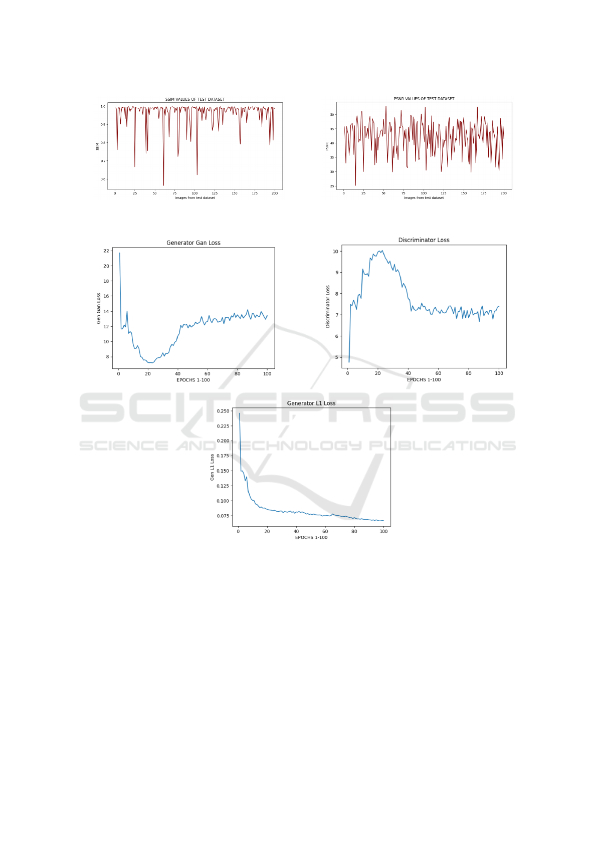
(a) SSIM values. (b) PSNR values.
Figure 7: SSIM and PSNR values between ground truth and predicted images from test dataset.
(a) Generator Gan Loss during training. (b) Discriminator Loss during training.
(c) Generator L1 Loss during training.
Figure 8: Comparison of losses.
REFERENCES
Acito, N. and Diani, M. (2018). Atmospheric column water
vapor retrieval from hyperspectral vnir data based on
low-rank subspace projection. IEEE Transactions on
Geoscience and Remote Sensing, 56(7):3924–3940.
Basener, B. and Basener, A. (2023). Gaussian process and
deep learning atmospheric correction. Remote Sens-
ing, 15(3):649.
Bernstein, L. S., Jin, X., Gregor, B., and Adler-Golden,
S. M. (2012). Quick atmospheric correction code: al-
gorithm description and recent upgrades. Optical en-
gineering, 51(11):111719–111719.
Hsu, N., Jeong, M.-J., Bettenhausen, C., Sayer, A., Hansell,
R., Seftor, C., Huang, J., and Tsay, S.-C. (2013). En-
hanced deep blue aerosol retrieval algorithm: The sec-
ond generation. Journal of Geophysical Research: At-
mospheres, 118(16):9296–9315.
Ilori, C. O. and Knudby, A. (2020). An approach
to minimize atmospheric correction error and im-
prove physics-based satellite-derived bathymetry in a
coastal environment. Remote Sensing, 12(17):2752.
Liu, S., Li, H., Jiang, C., and Feng, J. (2024). Spectral–
spatial graph convolutional network with dynamic-
synchronized multiscale features for few-shot hy-
perspectral image classification. Remote Sensing,
IC3Com 2024 - International Conference on Cognitive & Cloud Computing
184

16(5):895.
Liu, S., Zhang, Y., Zhao, L., Chen, X., Zhou, R., Zheng, F.,
Li, Z., Li, J., Yang, H., Li, H., et al. (2022). Quan-
titative and automatic atmospheric correction (quaac):
Application and validation. Sensors, 22(9):3280.
Phiri, D., Simwanda, M., Salekin, S., Nyirenda, V. R., Mu-
rayama, Y., and Ranagalage, M. (2020). Sentinel-2
data for land cover/use mapping: A review. Remote
Sensing, 12(14):2291.
Remer, L. A., Levy, R. C., Mattoo, S., Tanr
´
e, D., Gupta, P.,
Shi, Y., Sawyer, V., Munchak, L. A., Zhou, Y., Kim,
M., et al. (2020). The dark target algorithm for ob-
serving the global aerosol system: Past, present, and
future. Remote sensing, 12(18):2900.
Schl
¨
apfer, D., Borel, C. C., Keller, J., and Itten, K. I.
(1998). Atmospheric precorrected differential absorp-
tion technique to retrieve columnar water vapor. Re-
mote Sensing of Environment, 65(3):353–366.
Wang, Y., Hong, D., Sha, J., Gao, L., Liu, L., Zhang,
Y., and Rong, X. (2022). Spectral–spatial–temporal
transformers for hyperspectral image change detec-
tion. IEEE Transactions on Geoscience and Remote
Sensing, 60:1–14.
Zhang, H., Ma, Y., Zhang, J., Zhao, X., Zhang, X., and
Leng, Z. (2022). Atmospheric correction model for
water–land boundary adjacency effects in landsat-8
multispectral images and its impact on bathymetric re-
mote sensing. Remote Sensing, 14(19):4769.
Zhao, X., Ma, Y., Xiao, Y., Liu, J., Ding, J., Ye, X., and Liu,
R. (2023). Atmospheric correction algorithm based on
deep learning with spatial-spectral feature constraints
for broadband optical satellites: Examples from the
hy-1c coastal zone imager. ISPRS Journal of Pho-
togrammetry and Remote Sensing, 205:147–162.
Zhu, W. and Xia, W. (2023). Effects of atmospheric cor-
rection on remote sensing statistical inference in an
aquatic environment. Remote Sensing, 15(7):1907.
Atmospheric Correction of Sentinel-2 Images Using Deep Learning
185