Forecasting Annual Expenditure in E-Commerce

Abhijeet Yadav, Vinayak Shukla, Dilip Woad, Romil Raina and Himani Deshpande

Thadomal Shahani Engineering College, Bandra (West) Mumbai 400050, India

Keywords: E-Commerce, Expenditure, Support Vector Regression, Adaboost, XGBoost.

Abstract: With the rapid penetration of E-commerce in modern society, there is a need to have a holistic analysis of

annual expenditure forecasting in e-commerce, underscoring its importance to modern consumer behaviour

and economic growth. To achieve the same, this study explores seven machine learning based methodologies

namely linear regression, random forest, decision trees, K-Nearest Neighbors (KNN), AdaBoost, Support

Vector Regression (SVR), and XGBoost. Through an extensive examination of the effectiveness of each

model, this research aims to provide useful information on the effectiveness of used techniques towards

predicting yearly expenditures in a dynamic environment like e-commerce. These findings are important for

the stakeholders seeking to improve their management strategies in the e-commerce sector, where it is

necessary to understand consumers for sustainable development. Two different datasets namely Open Mart

and E-Mart are used, which provides expenditure data of various companies found within different regions

operating on e-commerce platforms. Among the used methodologies, the Linear Regression is found to be the

most efficient one on both datasets, with 97% and 89% prediction accuracy on the Open Mart dataset and the

E-Mart dataset, respectively. In contrast, Support Vector Regression (SVR) performs the worst on both the

datasets. In depth analysis of the datasets reveals a strong relationship between the increasing use of apps,

membership orders, and consumer expenditure overall. Thus, this study suggests that e-commerce companies

may increase revenue and consumer engagement by optimizing app usage and promoting membership

programs with the help of this insight.

1 INTRODUCTION

Accurate annual expenditure forecasting is essential

for businesses trying to navigate competitive markets

and maximize resource allocation in the ever-

changing world of e-commerce. This study explores

the field of e-commerce spending forecasting using a

multivariate regression analysis methodology that is

deemed reliable. This paper's primary goal is to

provide insights for businesses using in-depth

modelling and predictive analysis of e-commerce

projects. By understanding trends and drivers,

companies can make better decisions about budget

allocation, inventory, pricing strategy and marketing

campaigns.

In e-commerce, machine learning is beneficial

when there is dynamic pricing and it can raise your

KPIs. This is because of the ML algorithms'

capability to identify new patterns in data. Because

of this, those algorithms are always picking up new

knowledge and identifying new trends and needs.

This is why Machine Learning models are opposed

to straightforward price markdowns and are used by

online retailers in the e-commerce sector for dynamic

pricing. Predictive algorithms help online retailers to

find the best deal on a given product, which gives an

advantage to online retailers. The best pricing, which

also considers condition of the warehouse, can be

chosen, along with the offer and real-time discounts

displayed. In order to maximize sales and optimize

inventory, these are performed predictive modelling

of the consumer spending requires a thorough

investigation of the delicate relationships between

numerous elements and how those ties affect the

purchasing behaviour. This study is after

investigation revealed significant variables

influencing yearly spend, providing essential

information for companies trying to maximize their

marketing budgets.

Significantly, support vector regression (SVR)

performs noticeably worse, particularly for sleep,

which displayed a negative R2 score on one data set.

186

Yadav, A., Deshpande, H., Shukla, V., Woad, D. and Raina, R.

Forecasting Annual Expenditure in E-Commerce.

DOI: 10.5220/0013305100004646

Paper published under CC license (CC BY-NC-ND 4.0)

In Proceedings of the 1st International Conference on Cognitive & Cloud Computing (IC3Com 2024), pages 186-195

ISBN: 978-989-758-739-9

In contrast, linear regression stands out as a strong

model, displaying remarkable accuracies above 90%

throughout the data sets. Annual spend is heavily

influenced by variables like uptime, and users are

more likely to devote their maximum time and

resources to mobile applications than to websites. In

summary, this study aims to contribute to the field of

forecasting analytics for e-commerce by a

comprehensive analysis of annual spending

forecasts. By providing strategic guidance and

actionable insights, it aims to empower E-Commerce

businesses to succeed in an increasingly competitive

world.

2 LITERATURE REVIEW

Research in expenditure forecasting for e-commerce

emphasizes the critical role of predictive analytics

methodologies. This research emphasizes on various

regression analysis to uncover the best expenditure

patterns. In a study [1], which shows how different

demographics of age, gender and marital status affect

consumer spending, the data was collected from the

state of Jammu and Kashmir, India with a total of 234

participants. This research shows young male with

marital status as single have a higher chance of e-

shopping Which helps the e-commerce website to

distribute advertisements accordingly. For owners to

understand how the revenue is distributed among

different categories, in this study [2], for e-commerce

sales forecasting the researcher builds a Directed

Acyclic Graph Neural Network (DAGNN). DAGNN

is used in deep learning for building neural network

in which the layers are presented as a directed acyclic

graph. A DAGNN can take inputs from multiple

layers and can give output to multiple layers. This

will be useful for long-term forecasts of product wise

daily sales revenue. The created forecasting will help

the owner to accurately predict the sales of the

product category for up to three months ahead. E-

commerce has helped both retailers and customers in

terms of cost, as demonstrated in study [3], which

examines how online shopping affects retailers'

selling prices and consumers' purchasing costs. The

study compared an online store with an offline store

and found that online shopping resulted in lower

costs for both retailers and consumers. This shows

that both retailers and customers have benefited from

the impact of e-commerce. In this study [4], research

was conducted for forecasting Walmart sales using

various machine learning models. The goal of this

research was to implement various machine learning

classification algorithms on the sales data of Walmart

stores present across the United States of America.

Algorithms used are Gradient Boosting, Random

Forest and Extremely Randomized Tree (Extra Tree)

and where compared using MAE evaluation R2

Score. This study shows Random Forest performs the

best as compared to other algorithms with the highest

R^2 accuracy of (0.94) and minimum MAE value of

(1979.4). Research [5] discussed various machine

learning algorithms which are commonly used in

sales forecasting, aiming to find the best machine

learning model with a better business understanding.

Algorithms on which the research was conducted are

Random Forest, Support vector machine, Decision

trees, Naïve bayes and Neural networks. The selected

algorithms are compared based on their accuracies.

The study shows Random Forest has the highest

accuracy score of 85℅, making it the most suitable

for sales prediction. In this study [6], research was

conducted to predict the sales of products based on

different factors like past history, seasonal trends,

location and festivities, with the help of machine

learning algorithms. Researchers selected five

algorithms KNN, NV (Naïve bayes), SVR, RF

(Random Forest) and MLR (Multiple linear

regression). Selected algorithms are compared based

on their Root Mean Square Error (RMSE) value.

After evaluating different algorithms, the researchers

found out MLR gives the most accurate results with

an RMSE value of 1.32, which is the lowest as

compared to other algorithms, followed by SVR, RF

and KNN with RMSE values of 2.35, 2.51 and 2.58

respectively. The algorithm that performed the worst

was NV with an RMSE value of 7.02.

3 METHODOLOGY

This paper contains the predictive analysis on the E-

commerce dataset with different Machine Learning

models to analyze the best model for regression

analysis.

3.1 Flowchart of Model

This article analyzes two datasets to get insight

into E-commerce clients' spending habits. This study

investigates numerous features such as session

length, app/website usage, membership term, and

annual spending to find hidden underlying patterns.

In Figure 1, the Model examines the e-commerce

dataset in a systematic manner. Initially, relevant

statistics are acquired and checked to ensure their

Forecasting Annual Expenditure in E-Commerce

187

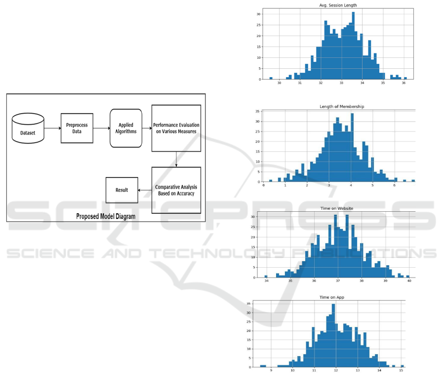
validity and applicability to real-world settings.

Second, the data is cleaned and organized to meet the

analytical requirements. Finally, numerous machine

learning algorithms are used to extract useful insights

from preprocessed data. The performance of these

algorithms is then rigorously assessed using several

assessment metrics. Finally, we compared and

analyzed the benefits and drawbacks of each

algorithm. Finally, our research presents the findings

from this systematic procedure, demonstrating the

effectiveness of various algorithms in identifying

patterns and practices in e-commerce. This sequential

procedure directs our inquiry and facilitates the

systematic analysis of e-commerce trends and

patterns.

Fig.1. Flow of Machine Learning Model.

The datasets used are readily available on platforms

like Kaggle and Github under the name ‘Ecommerce

Customers’, with no missing values for any features.

3.2 Exploratory Dataset Analysis

This section of the paper gives an insight to two

publicly available datasets which concerns patterns in

expenditure of buyers. Open Mart dataset which has

eight attributes out of which three are object data type

and rest are float data type. Email, Address and Avatar

are object data type and ‘Avg, Session Length’, ‘Time

on App’, ‘Time on Website’, ‘Length of Membership’

and ‘Yearly Amount Spent’ are float data types and

also an important numeric feature for further analysis.

The E-mart dataset has only numeric dataset, it has

total five numeric features namely Session length,

App Screentime, Website Screen Time, Number of

purchases and Yearly Amount Spent. Total number of

datapoints in Open mart and E-mart are 500 and 1000

respectively.

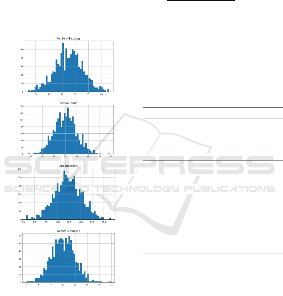
E-mart dataset has additional feature named ‘Number

of Purchases’ which is not available in Open Mart

dataset. Fig. 2 and Fig. 3, demonstrates the features of

both the datasets using histograms where x-axis

shows the time (in minutes) and y-axis shows number

of customers engaged in Session, App and Website

while purchasing. X-axis in the attribute ‘Length of

Membership’ shows time (in months) and for

‘Number of Purchases’ it is the total item purchased

by a specific user.

Fig .2. Histograms of different features in Open Mart

Dataset

Fig. 2(a) shows that the length of the sessions ranged from

about 20 to 40 minutes. Fig. 2(b) depicts that only few

people stay members for longer than five months, which

indicates that Open Mart is having trouble keeping clients

for long time. Fig.2 (c) and (d) shows consumers are

spending more time on the website than on the app. This

(a) Histogram of Avg. Session Length

(b) Histogram of Length of Membership

(c) Histogram of Time on Website

(d) Histogram of Time on App

IC3Com 2024 - International Conference on Cognitive & Cloud Computing

188

paper also analyses whether people are actually spending

more money on websites or apps with respect to Yearly

Amount Spent.

Fig. 3(b) shows that the length of the sessions ranged from

about 20 to 50 minutes. Fig. 3(b) shows that E-mart

customers are buying more items which indicates higher

shopping activity. Fig.3 (c) and (d) shows consumers are

spending even more time on the website and app.

(a) Histogram of Number of Purchases

(b) Histogram of Session Length

(c) Histogram of App Screentime

(d) Histogram of Website Screentime

Fig. 3. Histograms of different features in E-Mart Dataset

3.3 Identifying Correlation among

features

The Pearson correlation coefficient (r) is the method

to calculate the strength and direction of the linear

relationship between two variables in a correlation

analysis. The correlation coefficient can be

represented as in eq. (1):

𝑟=

∑

(𝑥



−𝑥̅)(𝑦



−𝑦)



∑

(𝑥



−𝑥̅)



∗∑(𝑦



−𝑦)



(1)

To identify the best correlating attribute, performed

correlation among the numeric features and

calculated coefficient of correlation(r). The

categorization of correlation coefficient for the

analysis is given below

r = 0 to 1 (Positively correlated)

r = 0 (No correlation)

r = -1 to 0 (Negatively Correlated)

Tabl e 1. Correlation table of E-commerce Open Mart

Dataset

Features R value

Length of Membership 0.8090

Time on App 0.4993

Avg. Session Length 0.3550

Time on Website -0.0026

Table 1 shows strong positive correlation of ‘Yearly

Amount Spent’ with ‘Length of Membership’ and

‘Time on App’ which shows Open Mart is

emphasizing on app optimization. While ‘Avg.

Session Length’ shows a moderate positive

correlation (0.3550). Least correlated feature is

‘Time on Website’ with r = -0.0026, it demonstrates

that website has no impact on annual spend.

Tabl e 2 . Correlation table of E-commerce E- Mart Dataset

Features R value

Number of Purchases 0.7791

App Screentime 0.6253

Session Length 0.6040

Website Screentime -0.3291

Table 2 shows strong positive correlation of ‘Yearly

Amount Spent’ with ‘Number of Purchases’ and

‘App Screentime’ which shows E-Mart is

emphasizing on product optimization. While

‘Session Length’ also shows a good positive

correlation (0.6040). Least correlated feature is

‘Website Screentime’ with r = -0.3291, it

Forecasting Annual Expenditure in E-Commerce

189

demonstrates that a website has minimal impact on

annual spent.

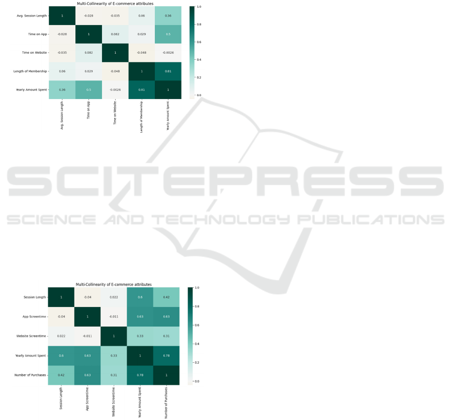
Below Fig. (4) represent correlation heatmaps

depicting the associations between features within

their respective datasets in the Open Mart dataset.

Heat maps are used to visualize and display a

geographic distribution of data as it represent

different densities of data points on a geographical

map to help in better analytic understanding.

Fig.4. Heat-map of different features in Open Mart dataset

In Open Mart dataset, Length of Membership

exhibits a positive correlation with r = 0.890 with the

dependent variable, indicating a strong relationship

as membership duration increases. Similarly, Time

on App shows a moderate positive correlation,

suggesting its influence on the dependent variable.

Time on Website demonstrates a negligible

correlation with the dependent variable.

Fig.5. Heat-map of different features in E- Mart dataset

Fig. (5) represents E-mart dataset, Number of

Purchases reveals a significant positive correlation

with the dependent variable. Moreover, both App

Screen Time and Session Length demonstrate

moderate positive correlations, indicating their

influence on the dependent variable. On the other

hand, Website Screen Time exhibits a negative

correlation with the dependent variable, suggesting

an inverse relationship.

An illustration of the relationship between a number

of independent attributes and our dependent feature

(annual amount spent) in the Open Mart Dataset in

Fig. (6).

Fig. (6), illustrates the strong positive correlation

between the parameters Length of Membership and

Time on App, while Time on Website exhibits the

most negative correlation. The features ‘Time on

App’ and ‘Length of Membership’ have a positive

correlation with ‘Yearly Amount Spent’ as the line

slopes upward from left to right. This implies that the

annual expenditure tends to increase together with

the increase of membership or app users. On the other

hand, if the line is horizontal that suggests no

correlation between variables as in Fig. 6 (b). Also, if

the data points cluster closely around the line, it

shows strong correlation as in Fig. 6 (a). Pictorial

representation of relationship between different

features with our dependent feature (Yearly Amount

Spent) for the E-mart Dataset in Fig. (7).

Fig. (7) illustrates the strong positive correlation

between the parameters App Screen Time and

Number of purchases while Website Screentime

exhibits the most negative correlation. The features

‘App Screentime’ and ‘Number of purchases’ have a

positive correlation with ‘Yearly Amount Spent’ as

the line slopes upward from left to right. This implies

that the annual expenditure tends to increase together

with the increase of quality product or app users.

Also, if the data points cluster closely around the line,

it shows strong correlation as in Fig. 7 (b) between

‘Number of Purchases’ and ‘Yearly Amount Spent’.

IC3Com 2024 - International Conference on Cognitive & Cloud Computing

190

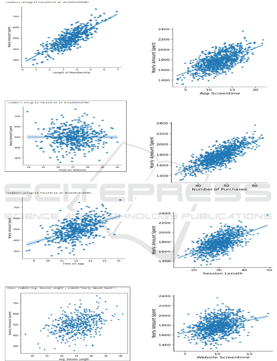
(a) Scatterplot of Length of Membership

(b) Scatterplot of Time on Website

(c) Scatterplot of Time on App

(d) Scatterplot of Avg. Session Length

Fig.6. Scatterplot between different features in Open Mart

Dataset

(a) Scatterplot of App Screentime

(b) Scatterplot of Number of Purchases

(c) Scatterplot of Session Length

(d) Scatterplot of Website Screentime

Fig.7. Scatterplot between different features in E- Mart

Dataset.

Forecasting Annual Expenditure in E-Commerce

191

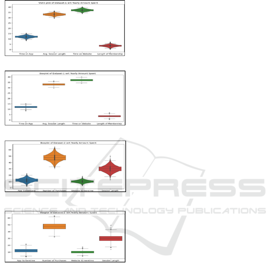
(a)

Violin Plot showing Open Mart Dataset

(b) Box Plot showing Open Mart Dataset

(c) Violin Plot showing E-Mart Dataset

(d) Box Plot showing E-Mart Dataset

Fig.8. Violin and Box plot depicting both datasets.

Fig (8). Shows the box and violin plot of respective

datasets where it shows important parameters like

mean, IQR (Inter-Quartile Range), minimum and

maximum value of datasets etc. Fig 8(a) and Fig. 8(b)

shows the customers spend 33 minutes a session on

average, with a median session length of 33.08

minutes. 25% of sessions last less than 32.34

minutes, according to the distribution, and 75% of

sessions last longer than 33.71 minutes. Customers

use the platform for an average of 12 minutes on the

mobile app and 37 minutes on the website, with

respective median times of roughly 12 and 37

minutes. With 25% of customers having a

membership term of less than 2.93 years and 75%

having a duration of more than 4.13 years, the length

of membership demonstrates a median duration of

almost 3.53 years. The study of E-mart dataset is

shown in Figs. 8(c) and 8(d), and it demonstrates that

customers spend about thirty minutes a session on

average, with an average of 12.21 minutes spent on

apps and 10.01 minutes spent on websites.

Furthermore, consumers spend $1778.73 annually on

purchases, or about 47.56 transactions annually on

average. It also shows that features like “Avg.

Session Length”, “Time on App”, “App Screentime”

the data cluster closely around their means, with

narrow IQR, indicating relatively consistent behavior

whereas “Time on Website” displays a wider spread

of values, suggesting more variability. “Length of

Membership" shows a moderate spread, with a longer

right tail indicating some customers with extended

memberships. "Yearly Amount Spent" exhibits a

right-skewed distribution, with most customers

spending lower amounts annually, but with notable

outliers spending significantly more.

3.4 Regression Methods

We have used seven important Machine Learning

models to perform regression on datasets namely

Linear Regression, Random Forest, Ada Boost,

Decision Tree, KNN, SVR, XG Boost.

a) Linear regression:

Linear Regression is a supervised ML model which

learns through labeled input and output data and used

for analysing the relationship between a dependent

variable and one or more independent variables as

expressed in equation (2). It predicts the best-fit line

to the data points., Linear Regression objective is to

minimize the difference between the observed and

predicted values.

𝑦=𝑎 𝑏𝑥 (2)

b) Random Forest Regression:

Random Forest is an ensemble learning approach that

successively constructs various ML models, such as

decision trees, during training and returns the mode

of classes for categorization or the average prediction

of the individual trees. It is an approach that

generates decision trees during training and then

combines their predictions. Overall, this prediction

improves model accuracy while reducing overfitting.

IC3Com 2024 - International Conference on Cognitive & Cloud Computing

192

c) AdaBoost

AdaBoost is an adaptive boosting algorithm that

combines multiple weak learners or ML models

sequentially to predict or classify. It is also an

ensemble learning technique which combines

multiple weak models sequentially to create a strong

model. It is specifically used for classification tasks.

d) Decision Tree

Decision Tree is a non-parametric supervised

learning method which means it does not make any

assumptions regarding the sample beforehand and

this method is used for classification and regression

and can handle both numerical and categorical data.

It has tree structure which consist of root node,

internal node and leaf nodes. Decision tree is mainly

used for classification purpose.

e) K-Nearest Neighbor (KNN)

KNN (K-Nearest Neighbors) is a non-parametric

technique that performs classification and regression

tasks without making any prior assumptions about

the sample. based on the average value or majority

class of its k closest neighbors in the feature space,

predicts the class or value of a new data point. It

employs many distance functions, such as the

Euclidean distance (represented in equation (3)), the

Manhattan distance (expressed in equation (4)), and

the Minkowski distance (expressed in equation (5)),

where q denotes the order of norm, to determine the

nearest neighbor.

𝐸.𝐷=



∑(

𝑥



−𝑦



)







(3)

𝑀.𝐷=

∑

𝑥



−𝑦



|





| (4)

𝑀𝑖𝑛𝑘.𝐷.=((|𝑥



−𝑦



|)



)





/

(5)

Where 𝑥



and 𝑦



represents the coordinates of x and

y datapoints on 𝑖



dimension and q the order of the

distance.

f) Support Vector Regression

SVR (Support Vector Regression) is a supervised

machine learning model used in regression purpose.

It includes the concept of hyperplane which classifies

data points in two separate classes. It finds the

optimal plane also called hyperplane to separate or

classify two datapoints into two different classes. It

aims to find a function that has a maximum margin

of tolerance to the given data points. SVR is

expressed in equation (6).

𝑆𝑉𝑅=𝑀𝐼𝑁

∑(

𝑦



−𝑤



𝑥



)





(6)

g) XG Boost

The XG Boost technique optimizes a differentiable

loss function for each iteration, such as the mean

squared error (MSE) for regression. It constructs

several decision trees one after the other, fixing the

mistakes of the first tree. It uses an objective function

regularization term to penalize and prevent

overfitting.

3.5 Result

This section of the paper depicts the experimental

results using the selected regression methods. Results

are evaluated on Four performance metrics namely

Mean Squared Error (MSE), Mean Absolute Error,

Root Mean Squared Error, R2(R-Squared). Mean

squared error is defined as the average of the absolute

squared difference between the output value and the

predicted value. MSE is represented as in equation

(7). Mean Absolute Error is defined as the average of

the absolute difference between the actual output and

the predicted output. Mathematically, its represented

as in equation (8). Root Mean Squared Error is

defined as the square root of the average of the

squared difference between the output value and the

predicted value. It can be represented as in equation

(9). R2 score represents the proportion of the

variance in the dependent variable that is explained

by the independent variables in the model.

Mathematically it is represented as in equation (10).

𝑀𝑆𝐸=

1

𝑁

(𝑦



−𝑦



)







(7)

𝑀𝐴𝐸=

1

𝑁

|𝑦



−𝑦



|







(8)

𝑅𝑀𝑆𝐸=



1

𝑁

(𝑦



−𝑦



)







(9)

𝑅



=1−

𝑆𝑆



𝑆𝑆



=1−

∑(

𝑥



−𝑥



)







∑(

𝑦



−𝑦



)







(10)

Forecasting Annual Expenditure in E-Commerce

193

Where 𝑦



and 𝑥



represents the predicted outcome on 𝑖



dimension.

Table.3. Experimental results on Open Mart Dataset

Algorithm MSE RMSE MAE R2

Linear

Regression

109.86 10.48 8.55 0.97

Random

Forest

337 18.36 14.04 0.93

AdaBoost 579.09 24.06 19.70 0.88

Decision

Tree

802 28.32 22.21 0.83

KNN 465.62 21.57 16.63 0.90

SVR 5024.6

7

70.88 54.33 -0.014

XG Boost 262.18 16.19 12.36 0.94

As shown in table 3, with the lowest Mean Squared

Error (MSE) of 109.86, Root Mean Squared Error

(RMSE) of 10.48, and Mean Absolute Error (MAE)

of 8.55, as well as the highest R-squared value (97%

accuracy), which demonstrates its superior predictive

capability, illustrates that Linear Regression is the

most accurate model in Open Mart dataset. With an

accuracy percentage of almost 94%, an MSE of

262.18, an RMSE of 16.19, an MAE of 12.36, and

competitive performance, XG Boost comes in close

second. Support Vector Regression (SVR), on the

other hand, performs the worst and has the worst

error metrics: 5024.67 MSE, 70.88 RMSE, 54.33

MAE, and an extremely low R-squared value, all of

which amply demonstrate SVR's inability to make

accurate predictions.

Table.4. Experimental results on E- Mart Dataset

Algorithm MSE RMSE MAE R2

Linear

Regression

2693.2

7

51.89 41.42 0.89

Random

Forest

3981.4

2

63.09 51.09 0.84

AdaBoost 4720.3

0

68.70 54.34 0.81

Decision

Tree

7749.0

1

88.02 69.65 0.69

KNN 4452.1

7

66.72 53.37 0.82

SVR 17593 132.64 102.32 0.30

XG Boost 4082.9

9

63.89 51.13 0.83

Experimental results on E-mart dataset suggests that

Linear regression is the best performing model when

it is evaluated against various machine learning

algorithms. Linear Regression has the lowest Mean

Squared Error (MSE) of 2693.27 and highest R-

squared value (89% accuracy), the lowest Root

Mean Squared Error (RMSE) of 51.89, and the

Mean Absolute Error (MAE) of 41.42. This shows

that, in comparison to other models, it has better

predicted accuracy and precision. As shown in table

4, XG Boost, comes second best with an MSE of

4082.99, RMSE of 63.89, MAE of 51.13, and an

accuracy percentage of almost 83%. Support Vector

Regression performs the worst out of all the models.

It has the highest error metrics, with an MSE of

17593, an RMSE of 132.64, an MAE of 102.32, and

a very relatively low R-squared value of 30%

accuracy only, which shows that it is not very good

at generalizing the patterns in the dataset.

4 CONCLUSION

Linear Regression is the best model with the

accuracy of greater than 90% in both the dataset.

Furthermore, XG Boost performs second best, with

accuracy and precision that are closely behind that of

Linear Regression. Support Vector Regression

(SVR), on the other hand, performs the worst out of

all the models. Its inability to forecast outcomes and

capture dataset patterns is highlighted by its high

error metrics and low R-squared values (30%) in E-

mart and negative R-squared value in Open Mart

Dataset

. This could me mainly due to potential nonlinear

relationships between the set of input features

together and the output variable.

These findings show

model effectiveness for e-commerce prediction tasks

.

After analysing the nuances of several attributes

and how they relate to each other in the datasets,

membership duration and app usage time are the

most important and significant factors affecting

annual yearly spending. Forecasting annual

expenditure of customers shows they prefer app than

website for shopping, so to cater large audience,

companies should focus to improve working of apps

and also offer some discounts and incentives to their

loyal customers. E-commerce Companies should

focus to improve and work on functioning of their

website as it is inversely correlated with annual

expenditure. They should improve the user interface

and other functionalities of website to make it more

IC3Com 2024 - International Conference on Cognitive & Cloud Computing

194

user friendly. Number of purchases is highly

positively correlated with annual expenditure which

tells about their good product quality and trust they

built with customers in term of quality assurance.

REFERENCES

Bhat, S.A., Islam, S.B. and Sheikh, A.H., 2021. Evaluating

the influence of consumer demographics on online

purchase intention: An E-Tail Perspective. Paradigm,

25(2), pp.141-160.

Petroșanu, D.M., Pîrjan, A., Căruţaşu, G., Tăbușcă, A.,

Zirra, D.L. and Perju-Mitran, A., 2022. E-Commerce

Sales Revenues Forecasting by Means of Dynamically

Designing, Developing and Validating a Directed

Acyclic Graph (DAG) Network for Deep Learning.

Electronics, 11(18), p.2940.

Miyatake, K., Nemoto, T., Nakaharai, S. and Hayashi, K.,

2016. Reduction in consumers’ purchasing cost by

online shopping. Transportation Research Procedia, 12,

pp.656-666.

Elias, N.S., & Singh, S. (2018). FORECASTING of

WALMART SALES using MACHINE LEARNING

ALGORITHMS.

Singh, K., Booma, P.M. and Eaganathan, U., 2020,

December. E-commerce system for sale prediction

using machine learning technique. In Journal of

Physics: Conference Series (Vol. 1712, No. 1, p.

012042). IOP Publishing.

"E-Commerce Sales Prediction", International Journal of

Emerging Technologies and Innovative Research

(www.jetir.org), ISSN:2349-5162, Vol.7, Issue 4, page

no.986-992, April-2020,

Ji, S.; Wang, X.; Zhao, W.; Guo, D. (2018) "An Application

of a Three-Stage XGboost-Based Model to Sales

Forecasting of a Cross-Border e- Commerce

Enterprise." Math. Probl. Eng. 8503252[1].

Liu, J.; Liu, C.; Zhang, L.; Xu, Y. (2020)"Research on Sales

Information Prediction System of E-Commerce

Enterprises Based on Time Series Model." Inf. Syst. e-

Bus. Manag., 18, 823–836[1].

Li, J.; Cui, T.; Yang, K.; Yuan, R.; He, L.; Li, M (2021)

"Demand Forecasting of E-Commerce Enterprises

Based on Horizontal Federated Learning from the

Perspective of Sustainable Sustainability., 13, 13050[3].

Zhang, X. (2020) "Prediction of Purchase Volume of Cross-

Border e- Commerce Platform Based on BP Neural

Network." Comput. Intell. Neurosci., 3821642[3].

Turóczy Z., Liviu Marian (2019) ‘Multiple regression

analysis of performance indicators in the ceramic

industry’

Micu, A., Geru, M., Capatina, A., Avram, C., Rusu, R. and

Panait, A.A., 2019. Leveraging e-Commerce

performance through machine learning algorithms.

Ann. Dunarea Jos Univ. Galati, 2, pp.162-

171.Prediction’

Sharma, M., Sharma, V. and Kapoor, R., 2022. Study of E-

Commerce and Impact of Machine Learning in E-

Commerce. In Empirical Research for Futuristic E-

Commerce Systems: Foundations and Applications (pp.

1-22). IGI Global.

Pavel J., Lenka V., Lucie S., Zdenek S., (2019) ‘Predictive

Performance of Customer Lifetime Value Models in E-

Commerce and the Use of Non-Financial Data’

Zhang, X., Guo, F., Chen, T., Pan, L., Beliakov, G. and Wu,

J., 2023. A Brief Survey of Machine Learning and Deep

Learning Techniques for E-Commerce Research.

Journal of Theoretical and Applied Electronic

Commerce Research, 18(4), pp.2188-2216.

Forecasting Annual Expenditure in E-Commerce

195