Hidden Markov Models to Capture Sequential Patterns of

Valence-Arousal in High- and Low-Performing Collaborative

Problem-Solving Groups

Yaping Xu

, Honghui Li

, Weitong Guo

1,* b

, Tian Feng

, Xiaonan Yin

, Sen Bao

and Lu Chen

School of Educational Technology, Northwest Normal University, Lanzhou, China

Faculty of Education, Beijing Normal University, Beijing, China

Keywords: Collaborative Problem-Solving, Dimensional Emotion, Machine Learning, Hidden Markov Model.

Abstract: Emotion is an important factor affecting students' cognitive processing and learning outcomes. Accurately

detecting the group members’ emotions in collaborative problem-solving environments is an important basis

for judging their learning status and providing personalized support. However, current research mainly

focuses on discrete emotions and lacks the identification and analysis of learning emotions from the

perspective of dimensional emotions, which may lead to an oversimplified representation of students'

emotions. Therefore, based on the circumplex model of affect, this study used multiple machine learning

methods to predict students' affective valence and arousal from facial behavioural clues when they participated

in online collaborative problem-solving activities. The results indicated that the random forest model

performed best. In order to enhance the understanding of the temporal nature of group emotions and their

relationship with CPS outcomes, we also applied hidden Markov models (HMMs) to reveal the differences in

sequential patterns between high- and low-performing groups. It was found that the sequential patterns of

affective valence-arousal in the two groups of students were quite different, and students in the high-

performing groups were more likely to regulate their emotions and transition to appropriate states (such as

states with positive valence or high arousal) to successfully solve problems. This study has important

methodological significance for the automatic measurement and analysis of dimensional emotions.

1 INTRODUCTION

Collaborative problem solving (CPS), as an essential

skill in the 21st century, is a ubiquitous form of

collaborative learning in higher education and can

promote active learning. It refers to two or more

students working in groups to share their skills and

knowledge to solve open-ended and ill-structured

problems (Hmelo-Silver and DeSimone 2013). CPS

not only includes cognitive processes but also

integrates the social process of collaborative

interaction. In addition, emotional factors are also an

important part.

Researchers generally believe that students'

affective states have an impact on online

collaborative problem-solving learning, and it,

together with cognitive factors, affects the outcomes

https://orcid.org/0009-0002-1091-6939

Corresponding Author: guowt@nwnu.edu.cn

https://orcid.org/0009-0006-9501-1010

of online collaborative problem-solving. For

example, Mandler (Mandler 1989) claims that

students' emotional reactions and physiological

experiences caused by challenges and obstacles are

closely related to problem-solving. According to

Mayer (Mayer 1998), non-cognitive factors such as

individual emotions and motivations, together with

cognitive factors such as knowledge and strategies,

influence the problem-solving process.

Most studies use discrete labels to characterize

students' emotions. However, people often show

subtle and complex affective states in daily

interactions, and it is difficult to accurately describe

students' emotions using only a few labels. Another

possibility is to characterize students’ emotions by

observing their dimensions. A popular theoretical

framework is the "circumplex model of affect"

proposed by Russell (Russell 1980), which holds that

Xu, Y., Li, H., Guo, W., Feng, T., Yin, X., Bao, S. and Chen, L.

Hidden Markov Models to Capture Sequential Patterns of Valence-Arousal in High- and Low-Performing Collaborative Problem-Solving Groups.

DOI: 10.5220/0013038900003932

Paper published under CC license (CC BY-NC-ND 4.0)

In Proceedings of the 17th International Conference on Computer Supported Education (CSEDU 2025) - Volume 1, pages 173-179

ISBN: 978-989-758-746-7; ISSN: 2184-5026

173

all emotions contain two dimensions: valence (from

negative to positive) and arousal (from relaxed to

excited). The dimensional approach can more

effectively describe students' complex emotions from

the perspective of emotion synthesizers. From the

current research, there is still a lack of empirical

exploration and in-depth research on the relationship

between dimensional emotions and online

collaborative problem-solving. Although existing

studies have paid some attention to the relationship

between the two, these studies have neither analysed

the relationship between group-level emotions and

CPS outcomes, nor ignored the interaction between

different dimensions.

Furthermore, the majority of previous studies

have measured emotional valence and arousal

through the use of conventional techniques like

questionnaires or observations. This approach is

unable to provide fine-grained process analysis and

cannot obtain the dynamic changes in students'

emotions during the learning process. With the

development of affective computing technology, new

analysis methods such as facial behaviour recognition

open up new avenues for studying students' emotional

responses in CPS environments (Hayashi 2019).

Therefore, this study aims to identify students'

emotional responses during the CPS process using an

automatic method and determine the affective

valence and arousal at the group level through a

voting strategy. Moreover, this study uses the HMM

method to explore the sequential patterns of

emotional responses and their relationship with CPS

outcomes. The study is guided by the following

research questions (RQs):

 RQ1: How can students' emotional responses

during the CPS process be automatically identified?

 RQ2: what is the relationship between the

emotional dimensions (valence and arousal) and

CPS outcomes?

2 LITERATURE REVIEW

2.1 Affective States in Collaborative

Problem-Solving Activities

CPS is a complex, multi-dimensional approach in

which learners collaborate to share their insights on a

problem and combine their knowledge, skills, and

efforts to seek solutions (Hmelo-Silver 2004; Fiore et

al. 2017). Throughout the problem-solving process,

discussions of varying viewpoints often arise, which

can lead to potential conflicts. As a result,

collaborative participants may express a wide range

of emotions. Both individual and collective emotional

states significantly influence behaviours and

interactions within the group (Schunk and

Zimmerman 2012).

From the viewpoint of dimensional emotions,

students engaged in collaborative groups experience

varying levels of valence and arousal, which

subsequently influence their learning processes and

outcomes. Research indicates that valence is linked to

cognitive flexibility, perceptual processing, and

creative problem-solving abilities (Isen 2015), while

arousal impacts attention and cognitive functioning

(Critchley, Eccles, and Garfinkel 2013). Given that

these dimensions define emotional responses and

directly affect learning, it is crucial to examine each

component thoroughly to grasp its expression and

effects in educational contexts. Regarding

individuals' emotional states during collaboration,

negative emotions are tied to disengagement and

social loafing, whereas deactivated positive emotions

(e.g., calm) correlate positively with group

interactions, and deactivated negative emotions (e.g.,

tired) show a negative relationship with group

dynamics (Linnenbrink-Garcia, Rogat, and Koskey

2011).

In conclusion, the emotions consistently present

during collaborative group interactions play a

significant role in shaping the learning process (Baker,

Andriessen, and Järvelä 2013). When individuals

work together in a group, it's likely that their affective

states align, resulting in shared and interactive

emotional experiences. Nevertheless, there is limited

research on the emotional evolution patterns of

groups as a whole.

2.2 Analysis Methods for Sequence

Data

Sequence analysis methods are increasingly being

used to analyse longitudinal data consisting of

multiple independent subjects. The methods that rely

on the sequence characteristics of data for analysis

and mining also exist in the literature in the field of

education. For example, some studies have

predominantly used lag sequential analysis to explore

the temporal patterns of group learning engagement

(Hou and Wu 2011; Tao et al. 2022); however, this

approach has failed to reveal the interconnections

among different dimensions. Compared with the

analysis method, the advantage of HMM is that it can

extract simplified hidden states and their transition

relationships and can process multi-channel data.

In the Hidden Markov Model, sequence data

consists of observed states, which are considered

CSEDU 2025 - 17th International Conference on Computer Supported Education

174

probability functions of hidden states. The hidden

states cannot be observed directly but can be inferred

from the observed sequence. The transition

probabilities of hidden states reflect the temporal

characteristics. In terms of multi-channel data, the

same latent structure is captured for all channels. If

there is missing data in some channels, the multi-

channel method is still useful and the data can be used

as is. Overall, HMM is suitable for processing two-

channel valence-arousal data due to its various

advantages in this study. It exhibited the potential to

capture the interplay among the two dimensions of

students’ emotions and to understand how emotions

change over time.

3 METHODOLOGY

3.1 Participants and Context

This study involved 54 undergraduate students (46

females, and 8 males; aged 20-25 years) who come

from the same normal university in Beijing, China.

The participants have various majors, including

educational technology, psychology, statistics, and

physics. They were assigned into 18 groups based on

major. Each group was asked to complete an online

collaborative problem-solving activity with the theme

of “Migration of Migrant Workers”, predicting the

trend of population changes while taking into account

a number of variables. Before the activity, all students

were informed of the content and procedure of the

study, and their rights to withdraw from the research

at any time. In addition, the researchers promised the

participants that all collected data would be strictly

confidential and used only for research purposes.

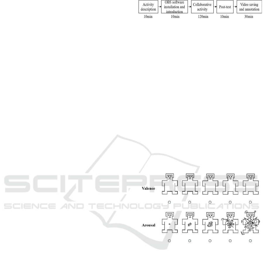
3.2 Procedure

The activity process is depicted in Figure 1. First, the

researcher explained the procedure and requirements

of the collaborative activity. Each group member was

asked to install Open Broadcaster Software (OBS), a

cross-platform and open-source software that is

suitable for live streaming and recording. During the

activity, each group was given 120min complete the

collaborative task in a designated Tencent Meeting

room, writing a paper of approximately 1,000 words

presenting their solution to the problems. At the same

time, participants should use OBS software to video-

record their facial behaviours. The frame rate and

resolution of the videos were set to 20 and 512 × 288,

respectively. After the activity, participants need to

take a post-test and finish video annotation.

Figure 1: The process of the collaborative problem-solving

activity.

When a group completes learning tasks, each

member needs to upload their recorded videos to a

free cloud storage space. The researchers downloaded

the videos and cut them to obtain 20-minute video

clips. The video clips were then sent to the

corresponding student, who would annotate them

using the annotation tool. To be specific, each student

used the annotation tool to play their own video clips,

and the pop-up windows appeared automatically

every 30 seconds, displaying the valence-arousal

items using a 5-point Likert scale (see Figure 2). To

ensure the reliability of the annotations, students were

required to immediately rate and annotate the level of

valence and arousal in each 30-s clip according to the

actual situation at the time. This immediate

annotation procedure was implemented to minimize

memory bias and enhance the accuracy of the ratings.

Finally, timestamps and affective tags of each 30-s

clip were automatically saved in a CSV file.

Figure 2: A scale used to assess affective valence and

arousal.

3.3 Data Collection and Preprocessing

Papers submitted were used to measure the group's

performance. Each paper contained the group's

solution to three experimental problems: (1) Based on

the materials and data provided, a multiple regression

model was constructed to predict the change of

population in a city from 2023 to 2028; (2) The

reasons for the result in (1) were given; (3) Put

forward effective measures to attract the young

people to the city. To measure the group performance,

the researchers developed the scoring rubric

according to the mathematical abilities (Medová,

Bulková, and Čeretková 2020). Four components

were included in the rubric: typography, model

Hidden Markov Models to Capture Sequential Patterns of Valence-Arousal in High- and Low-Performing Collaborative Problem-Solving

Groups

175

building, application, and testing. Each component

was given a score ranging from 0 to 5, and the sum of

all component scores determined the paper's final

score. All papers were rated by two researchers who

have acquired training in using a scoring rubric. Then,

we ranked the groups from high to low based on the

mean scores of their papers. In line with prior studies

(Kelley 1939), groups that scored in the top 27% were

divided into the high-performing (HP) groups (N=5)

and those that scored in the bottom 27% were low-

performing (LP) groups (N=5).

As mentioned before, the facial behaviours of the

group members were video-recorded during the

collaborative task, and the participants subsequently

annotated the affective valence and arousal of some

clips in their own videos for training the machine

learning model. We found that 53 students (one

student dropped out of the labelling task) reported

their valence-arousal level 4240 times in total. We

aligned the intervals between self-reports with the

corresponding recorded videos based on the saved

timestamps and divided the videos into 30-s clips,

resulting in a total of 4240 video clips, each with two

labels: valence and arousal.

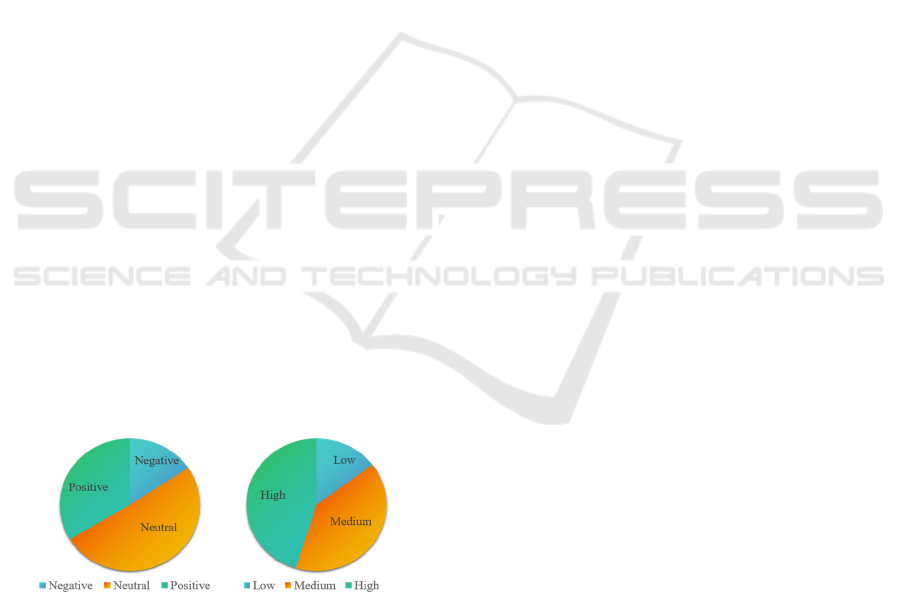
The statistical results show that video clips with

extremely low and high valence-arousal levels are

rarely observed. In order to make the labels more

balanced, we quantized the five-level labels into

low/negative, medium/neutral, and high/positive

groups. Figure 3 depicts the distribution of data with

different labels in valence and arousal. It can be seen

that the data remains imbalanced, which may cause

machine learning methods to produce biased

prediction results by ignoring minority classes. Thus,

a method named SMOTE-Tomek was used to handle

data imbalance in this study (Swana, Doorsamy, and

Bokoro 2022).

Figure 3: The distribution of data with different labels in

valence and arousal.

After the data processing was completed, we

adopted the technical route of feature extraction,

feature selection, and model training to obtain the

valence and arousal evaluation model. Firstly, we

used the open-source tool OpenFace 2.0 to extract

facial features from the students’ video clips. Then, a

feature selection method was utilized to select an

optimal feature subset from the original feature

vector. Finally, six machine learning classification

algorithms, including k-nearest Neighbor (KNN),

Decision Tree (DT), Naïve Bayes (NB), Support

Vector Machine (SVM), Logistics Regression (LR),

and Random Forest (RF), were applied to selected

features to train valence and arousal detection

models. The performance of these machine learning

algorithms was compared by checking the macro

precision(macro-P), macro recall(macro-R), macro

F1 score(macro-F1), and accuracy.

Once the best classification model is determined,

it can be used to automatically detect each student’s

affective valence (i.e., positive, neutral, negative) and

arousal level (i.e., high, medium, low) at each 30-s

clip. The group's valence and arousal level were then

measured at each 30-s clip through the use of a voting

strategy. For instance, the group is high-level arousal

if two or three members are. Note that the group's

label is classified as medium level in cases where

three members have inconsistent labels.

3.4 Hidden Markov Model

For each group, we would eventually obtain two sets

of sequence data reflecting changes in valence and

arousal levels, respectively. Time-varying processes

can be represented using Hidden Markov Model

(HMM) in a statistical or probabilistic framework.

The HMM approach was employed to describe a

Markov Chain with implicit unknown parameters,

uncover latent states within sequence data, and

capture the transition patterns between states that are

not observable in the sequences (Eddy 1996).

Compared with other sequence analysis approaches

(e.g. lag sequence analysis), it excels in handling

multi-channel sequence data.

In this study, the seqHMM package in R (Helske

and Helske 2019) can be used to analyse the two-

channel valence-arousal data and construct distinct

HMM models for the LP and HP groups, respectively.

The Expectation Maximization (EM) algorithm was

used with 100 iterations to fit and estimate HMM

models for both groups. The ideal number of hidden

states in each HMM model was determined by using

the Bayesian information criterion (BIC). More

specifically, we pre-specified the number of states in

the HMM model, ranging from 2 to 8. BIC value was

utilized as the measure of fit to determine the optimal

number of hidden states, with lower values indicating

a better fit. Furthermore, the seqHMM package was

used to graphically display the latent structures that

were found in both groups by visualizing hidden

states and transition modes.

CSEDU 2025 - 17th International Conference on Computer Supported Education

176

4 RESULTS AND DISCUSSION

4.1 Performance Analysis of Machine

Learning Models

For each 30-s video clip, 62-dimensional facial

features, including three types of facial behaviours—

facial action units, eye gaze, and head posture, were

extracted through OpenFace 2.0. After further feature

selection, 19 and 20 facial features were finally used

to train the valence and arousal assessment models,

respectively. To prevent overfitting, 80% of the

feature set was randomly selected for training and

20% for validation. There was no overlap between the

samples in the training set and the validation set. In

addition, the ten-fold cross-validation was applied to

evaluate models during the training process.

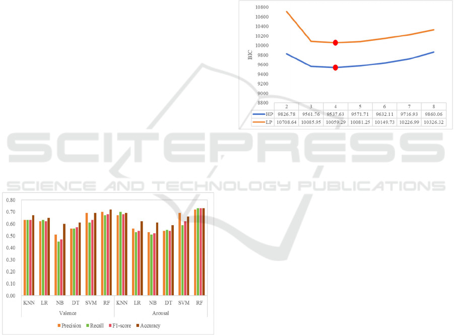
The indicators calculated by different methods are

shown in Figure 4. It can be seen that RF (Random

Forest) is superior to other algorithms in all metrics,

with accuracy of 0.72 and 0.76 in the valence and

arousal dimensions, respectively, indicating that the

RF model is the best-performing model overall. The

results of this study show that it is feasible and

effective to use computer vision technology to

automatically identify students' affective valence and

arousal levels during collaborative learning.

Therefore, the trained RF model was applied to

measure the remaining video clips for subsequent

analysis.

Figure 4: Classification results of different models in

valence and arousal dimension.

4.2 Sequential Patterns of Affective

Valence and Arousal Between the

HP and LP Groups

The RF model was used to detect students' affective

valence (positive, neutral, negative) and arousal level

(high, medium, low) in 30-second steps. For each

dimension, a 2-hour learning activity was able to

generate 240 values. With the video start time of

group members aligned, a voting strategy was used to

determine group-level valence and arousal levels in

each 30-s clip based on members' emotional

responses. In order to mine the hidden states and state

transition patterns that cannot be observed in

sequence data, HMM was used in this study. We set

2 to 8 states to fit the HMM models to the data and

used the BIC to determine which model best fits the

data, with lower values indicating better model fits

(see Figure 5). It was found that the 4-state model best

fit the data for both HP (BIC 9537.63) and LP groups

(BIC 10059.29).

Figure 5: Model fit (BIC) for 3 through 25 state models.

The structure of the best-fitting HMM was plotted

in Figure 6. The pies stand for the hidden states and

the slices represent the probabilities of the observed

states within each hidden state. The labels below

represent codes observed from both dimensions at the

same time (probability < 0.05 not shown). The arrows

between pies represent the transition direction and

probabilities, the greater the arrow's thickness, the

higher the probability. The results of the HMMs

revealed different sequential patterns in learning

emotions between the HP and LP groups.

Specifically, while the initial state for both the HP and

LP groups was neutral valence and medium-level

arousal, the HP groups showed a greater possibility of

transitioning to the second state, in which participants

experienced a higher level of arousal. It was also

easier for the HP groups to go from their last state to

their third one. In other words, negative emotions

with medium-level arousal of students from the HP

groups were more easily transferred to positive

emotions with high arousal. Moreover, the second

state and the fourth state in the LP group had a greater

probability of moving to each other.

Hidden Markov Models to Capture Sequential Patterns of Valence-Arousal in High- and Low-Performing Collaborative Problem-Solving

Groups

177

Figure 6: The HMM results of HP and LP groups.

The main findings of the study could provide new

insights into explaining the differences in

collaboration outcomes. This research emphasizes the

automatic detection of learners' affective states. By

identifying and distinguishing between arousal and

valence, this research goes beyond general emotional

recognition, allowing for a deeper understanding of

how these dimensions interact. The relationship

between these two dimensions was explored to offer

a more nuanced view of emotional regulation in

collaborative settings. This is not only beneficial for

teachers to provide just-in-time support, but also for

students themselves to become more aware of their

emotional states during the collaboration process.

This increased self-awareness can help students

regulate their own arousal levels and emotional

valence, leading to more effective and engaging

collaborative learning experiences.

5 CONCLUSION AND FUTURE

WORK

Learning emotions are closely related to academic

performance and have received extensive attention

from educational researchers. However, due to the

diversity of online learning environments and the

difficulty in directly observing students' learning

states, it is still extremely challenging to accurately

identify their affective states without interfering with

students. Therefore, this study analysed students'

facial behaviours and achieved automatic detection of

learning emotions from the perspective of

dimensional emotions based on computer vision

technology. The results show that identifying

students' affective states through facial behavioural

clues is an effective and non-invasive method. In

addition, we applied hidden Markov models to reveal

different sequential patterns of valence-arousal in

different performance groups. The results show that

compared with students in the LP groups, students in

the HP groups are more likely to move to a positive

or high arousal state. In the future, facial videos can

be added to the intelligent teaching system to build an

automatic emotion recognition function and provide

real-time feedback to teachers. With the support of

this function, teachers can monitor the changes in

students' emotional valence and arousal, change

teaching strategies in a timely manner, and provide

students with personalized feedback or intervention

measures so that students can regulate their emotions

and move to appropriate states (e.g. states with a

positive valence or high arousal) to achieve success

in problem-solving.

However, this study also has some limitations.

Firstly, it mainly relied on facial video data to

measure groups’ learning emotions. Although facial

expressions contain lots of emotional information, the

fusion of multimodal data can represent more

comprehensive information and train more accurate

emotion recognition models (Siddiqui et al. 2022).

Future research needs to collect information from

different channels (such as voice, gestures, body

posture, and physiological signals) and explore

effective fusion strategies to improve the accuracy of

emotion recognition models. In addition, regarding

the assessment of affective valence and arousal, this

study only used students’ facial videos in

collaborative problem-solving environments to train

models, which may affect the generalization ability of

models to a certain extent. Future research can collect

data from a wider range of collaboration scenarios to

train models.

ACKNOWLEDGEMENTS

This work was supported by the National Natural

Science Foundation of China (Grant No: 62267008).

REFERENCES

Baker, M., Andriessen, J., & Järvelä, S. (2013). Affective

learning together: Social and emotional dimensions of

collaborative learning. Abingdon, England: Routledge.

Critchley, H. D., Eccles, J., & Garfinkel, S. N. (2013).

Interaction between cognition, emotion, and the

autonomic nervous system. In Handbook of Clinical

Neurology, 117, 59-77. https://doi.org/10.1016/B978-

0-444-53491-0.00006-7.

Eddy, S. R. (1996). Hidden markov models. Current

Opinion in Structural Biology, 6(3), 361-365.

https://doi.org/10.1016/S0959-440X(96)80056-X.

Fiore, S. M., Graesser, A., Greiff, S., Griffin, P., Gong, B.,

Kyllonen, P., Rothman, R. (2017). Collaborative

problem solving: Considerations for the national

assessment of educational progress. Alexandria, VA:

National Center for Education Statistics.

CSEDU 2025 - 17th International Conference on Computer Supported Education

178

Hayashi, Y. (2019). Detecting collaborative learning

through emotions: An investigation using facial

expression recognition. In Intelligent Tutoring Systems:

15th International Conference (pp. 89-98). Springer

International Publishing. https://doi.org/10.1007/978-

3-030-22244-4_12.

Helske, S., & Helske, J. (2019). Mixture hidden markov

models for sequence data: The seqHMM package in R.

Journal of Statistical Software, 88(3), 1-32.

https://doi.org/10.18637/jss.v088.i03.

Hmelo-Silver, C. E. (2004). Problem-based learning: What

and how do students learn? Educational Psychology

Review, 16, 235-266. https://doi.org/10.1023/B:EDPR.

0000034022.16470.f3

Hmelo-Silver, C. E., & DeSimone, C. (2013). Problem-

based learning: An instructional model of collaborative

learning. In The International Handbook of

Collaborative Learning (pp. 370-385). Routledge.

Hou, H. T., & Sheng-Yi W. (2011). Analyzing the social

knowledge construction behavioral patterns of an

online synchronous collaborative discussion

instructional activity using an instant messaging tool: A

case study. Computers & Education, 57, 1459-1468.

https://doi.org/10.1016/j.compedu.2011.02.012.

Isen, A. M. (2015). On the relationship between affect and

creative problem solving. In Affect, Creative

Experience, and Psychological Adjustment (pp. 3-17).

Routledge.

Kelley, T. L. (1939). The selection of upper and lower

groups for the validation of test items. Journal of

Educational Psychology, 30(1), 17. https://doi.

org/10.1037/h0057123.

Linnenbrink-Garcia, L., Rogat, T. K., & Koskey, K. L.

(2011). Affect and engagement during small group

instruction. Contemporary Educational Psychology,

36(1), 13-24. https://doi.org/10.1016/j.cedpsych.

2010.09.001.

Mandler, G. (1989). Affect and learning: Causes and

consequences of emotional interactions. // Affect and

mathematical problem solving: A new perspective.

New York, NY: Springer, 3-19.

Mayer, R. E. (1998). Cognitive, metacognitive, and

motivational aspects of problem solving. Instructional

Science, 26, 49-63. https://doi.org/10.1023/A:

1003088013286.

Medová, J., Bulková, K. O., & Čeretková, S. (2020).

Relations between generalization, reasoning and

combinatorial thinking in solving mathematical open-

ended problems within mathematical contest.

Mathematics, 8(12), 2257. https://doi.org/10.

3390/math8122257.

Russell, J. A. (1980). A circumplex model of affect. Journal

of Personality and Social Psychology, 39(6), 1161.

https://doi.org/10.1037/h0077714.

Schunk, D. H., & Zimmerman, B. J. (2012). Motivation and

self-regulated learning: Theory, research, and

applications. Routledge.

Siddiqui, M. F. H., Parashar, D., Yang, X. L., & Ahmad, Y.

J. (2022). A survey on databases for multimodal

emotion recognition and an introduction to the VIRI

(Visible and InfraRed Image) database. Multimodal

Technologies and Interaction, 6(6): 47.

https://doi.org/10.3390/mti6060047.

Swana, E. F., Doorsamy, W., & Bokoro, P. (2022). Tomek

link and SMOTE approaches for machine fault

classification with an imbalanced dataset. Sensors,

22(9), 3246. https://doi.org/10.3390/s22093246.

Tao, Y., Zhang, M., Su, Y., & Li, Y. (2022). Exploring

college english language learners’ social knowledge

construction and socio-emotional interactions during

computer-supported collaborative writing activities.

The Asia-Pacific Education Researcher, 31: 613-22.

https://doi.org/10.1007/s40299-021-00612-7.

Hidden Markov Models to Capture Sequential Patterns of Valence-Arousal in High- and Low-Performing Collaborative Problem-Solving

Groups

179