Comparison Between Machine Learning and Deep Learning on Multiple
Motor Imagery Paradigms in a Low-Resource Context
Langlois Quentin
a
and Jodogne S
´
ebastien
b
Institute for Information and Communication Technologies, Electronics and Applied Mathematics (ICTEAM),
UCLouvain, Belgium
Keywords:
Deep Learning, Machine Learning, Neurophysiological Signals, Brain Computer Interface.
Abstract:
Motor Imagery (MI) decoding is a task aimed at interpreting the mental imagination of movement without any
physical action. MI decoding is typically performed through automated analysis of electroencephalographic
(EEG) signals, which capture electrical activity of the brain via electrodes placed on the scalp. MI decoding
holds significant potential for controlling devices or assisting in patient rehabilitation. In recent years, Deep
Learning (DL) techniques have been extensively studied in the MI decoding domain, often outperforming
traditional Machine Learning (ML) methods. However, these DL models are known to require large amounts
of data to achieve good results and substantial computational resources, limiting their applicability in low-
data or low-resource contexts. This work explores these assumptions by comparing state-of-the-art ML and
DL models under simulated low-resource conditions. Experiments were conducted on the Kaya2018 dataset,
enabling this comparison across multiple MI paradigms, which contrasts with other studies that typically focus
only on left/right-hand decoding task. The results indicate that even with limited data, DL models consistently
outperform ML techniques across all evaluated MI tasks, with the most significant advantage observed in
advanced experimental setups.
1 INTRODUCTION
Motor Imagery (MI) is a mental process in which
an individual imagines an action without performing
any physical movement (Mulder, 2007). Motor Im-
agery Brain-Computer Interfaces (MI-BCIs) are sys-
tems that leverage Artificial Intelligence (AI) to au-
tomatically decode the imagined action based on the
subject’s brain activity. MI-BCIs can be applied to a
wide range of practical applications, not only in the
medical domain to aid patient rehabilitation but also
for healthy individuals in video games or device con-
trol. MI decoding is typically based on the automated
analysis of electroencephalograms (EEG) (Lebedev
and Nicolelis, 2017), which capture the electrical ac-
tivity of the brain through electrodes placed on the
scalp. One major challenge is that EEG is a non-
stationary signal (Gramfort et al., 2013), meaning its
statistical properties vary across subjects and even
within the same subject over time. This limitation is
currently addressed by performing a dedicated cali-
bration of the MI decoding model before each new
a
https://orcid.org/0009-0006-7135-3809
b
https://orcid.org/0000-0001-6685-7398
usage of the MI-BCI system, which requires an ap-
propriate data collection protocol (Angulo-Sherman
and Guti
´
errez, 2014). However, this calibration is a
time- and energy-consuming task for the subject, lim-
iting the amount of data available to train the model.
To reduce this calibration procedure, a common
strategy is to leverage Machine Learning (ML) mod-
els, as they are fast and easy to train on standard
devices with limited amounts of data. However, it
has been shown that by using such models, between
10% and 50% of the population suffer from a so-
called “BCI inefficiency” (Alkoby et al., 2017). BCI-
inefficient users are unable to achieve BCI control, de-
fined as a final performance higher than 70% in the
left/right hand discrimination task, regardless of the
amount of training data.
In recent years, Deep Learning (DL) models (Le-
Cun et al., 2015) have been extensively stud-
ied, demonstrating higher performance than tradi-
tional ML models for BCI, especially among BCI-
inefficient users (Tibrewal et al., 2022). Further-
more, P
´
erez-Velasco et al. have recently demon-
strated that DL models can achieve BCI control in
more than 95% of subjects in a Leave-One-Subject-
704
Quentin, L. and Sébastien, J.
Comparison Between Machine Learning and Deep Learning on Multiple Motor Imagery Paradigms in a Low-Resource Context.
DOI: 10.5220/0013077600003911
Paper published under CC license (CC BY-NC-ND 4.0)
In Proceedings of the 18th International Joint Conference on Biomedical Engineering Systems and Technologies (BIOSTEC 2025) - Volume 1, pages 704-715
ISBN: 978-989-758-731-3; ISSN: 2184-4305
Proceedings Copyright © 2025 by SCITEPRESS – Science and Technology Publications, Lda.

Table 1: Number of sessions performed by each subject for each paradigm.
Paradigm Subject ID Total
(# subjects) A B C D E F G H I J K L M
5F (8) 2 4 2 0 3 3 2 1 2 0 0 0 0 19
CLA (7) 1 3 3 1 3 3 0 0 0 3 0 0 0 17
FreeForm (2) 0 1 2 0 0 0 0 0 0 0 0 0 0 3
HaLT (12) 3 3 2 0 3 3 3 2 2 1 2 2 3 29
NoMT (7) 0 0 0 0 0 1 0 1 1 1 1 1 1 7
Total 6 11 9 1 9 10 5 4 5 5 3 3 4 75
Out (LOSO) setting, based on a combination of mul-
tiple MI datasets (P
´
erez-Velasco et al., 2022). How-
ever, this study required training the model on EEG
data from 280 subjects and was limited to the binary
left/right hand MI task. Such extensive training de-
mands large amounts of data and dedicated hardware
infrastructure, which are typically unavailable in most
practical settings.
In contrast, this work explores the ability of DL
models to be calibrated with a limited amount of
data and compares these results against traditional
ML approaches. This comparison is based on the
Kaya et al. dataset (Kaya et al., 2018), allowing
the evaluation across multiple MI-BCI paradigms, be-
sides the regular left/right hand task. The ML clas-
sifiers compared are Linear Discriminant Analysis
(LDA), Support Vector Machine (SVM) (Hearst et al.,
1998), Random Forests (RF) (Breiman, 2001), and K-
Nearest Neighbors (K-NN). The compared state-of-
the-art DL architectures consist in EEGNet (Lawhern
et al., 2016), EEG-TCNet (Ingolfsson et al., 2020),
TCNet-Fusion (Musallam et al., 2021), and ATC-
Net (Altaheri et al., 2023). All these models have
been independently re-implemented and evaluated in
a strictly equivalent way, based on the within-subject
and LOSO methodologies. This approach enables an
objective and fair comparison of the ability of these
models to achieve high-quality results with limited
training data, as well as their capacity to benefit from
larger amounts of data. Finally, a time-based bench-
mark is proposed to compare their respective train-
ing/prediction rates, evaluating their suitability for
real-world applications.
2 MATERIALS AND METHODS
This section describes the experimental settings, in-
cluding the dataset, the data processing pipeline, the
training/evaluation methodologies, the ML classifiers,
as well as the DL models.
Table 2: Labels for each studied paradigm.
Paradigm labels
5F tumb, index, major, ring and pinkie fingers (right hand)
CLA left hand, neutral, right hand
HaLT left hand, left leg, neutral, right hand, right leg, tongue
2.1 Dataset
The dataset considered in this work is the Kaya2018
dataset (Kaya et al., 2018), which covers five different
MI paradigms: Classical (CLA), Hand-Legs-Tongue
(HaLT), 5-Fingers (5F), FreeForm, and NoMT, each
corresponding to a specific set of MI actions. The
dataset contains a total of 75 sessions recorded at
200 Hz
1
with a 21-channel EEG headset, involving
a total of 13 participants (identified by the letters A
through M). Each session contains 3 segments of 300
MI trials of approximately 3 seconds each (1 second
of MI followed by a 2-second break). Table 1 pro-
vides a summary of the total number of sessions per-
formed by each participant for each paradigm. The
labels identifying each paradigm are summarized in
Table 2. As the NoMT paradigm corresponds to no
motor imagination and the FreeForm paradigm was
only performed 3 times, they were not used in this
work. To accurately reproduce the data validation re-
sults from Kaya et al., a window of 170 EEG samples
(0.85 seconds at the rate of 200Hz) was used for each
MI trial.
2.2 Data Processing Pipeline
The provided data is already filtered using a band-
pass filter with a frequency range of 0.53 to 70 Hz,
with an additional 50 Hz notch filter to reduce electri-
cal grid interference. In this work, no further filtering
was applied to ensure consistency with the results re-
ported in the original paper. However, ML algorithms
typically require additional feature extraction steps to
achieve high-quality results. Therefore, the process-
ing pipeline developed by Mishchenko et al. has been
1
Some sessions were recorded at 1000 Hz but were re-
sampled to 200 Hz for data consistency.
Comparison Between Machine Learning and Deep Learning on Multiple Motor Imagery Paradigms in a Low-Resource Context
705

employed in this work (Mishchenko et al., 2019). The
same pipeline has previously been used by Kaya et al.
for their data validation procedure (Kaya et al., 2018).
This pipeline involves computing a 170-point Dis-
crete Fourier Transform (DFT), producing 86 com-
plex Fourier Transform Amplitudes (FTAs) for each
channel, spanning the frequency range with a granu-
larity of 1.18 Hz. Additionally, a low-pass 5 Hz filter
was applied by retaining the 5 lowest amplitudes (in-
cluding 0 Hz). Finally, these amplitudes were con-
verted to real values by concatenating the real and
imaginary parts (except for 0 Hz, which is always
real), resulting in a 9-value vector for each channel.
In contrast, DL models are known to achieve high-
quality results without extensive data processing. To
ensure a fair comparison between ML and DL ap-
proaches, all ML and DL models were evaluated both
with and without the FTA processing. For the DL
models, the input data was not flattened, as all tested
architectures expect a time dimension. For the ML
models, the vectors associated with each EEG chan-
nel were flattened to produce a 189-feature vector
with FTA and a 3,570-feature vector for raw signals.
Experiments have shown that only the LDA and k-
NN classifiers achieved better performance with FTA
processing.
2.3 Evaluation Methodologies
The baseline used in this work is an independent re-
production of the results of the original paper (Kaya
et al., 2018). This reproduction provides a robust,
validated baseline for comparing ML and DL models
across different setups, highlighting their respective
strengths and weaknesses. To this end, all ML and
DL models were independently re-implemented and
evaluated on each MI paradigm using three distinct
training/evaluation methodologies, each designed to
address specific challenges in EEG analysis:
1. Within-Subject, Single-Session. This setup
replicates the methodology of Kaya et al. by
training and evaluating models on a single ses-
sion from a specific subject. This methodology
was also used to simulate a few-shot learning sce-
nario by restricting the amount of training data.
The results for this setup can be found in the right
column of Figures 3 through 5 in the original pa-
per (Kaya et al., 2018).
It is important to distinguish this few-shot learn-
ing procedure from the recently introduced few-
shot transfer learning methodology (Mammone
et al., 2024). In few-shot transfer learning, DL
models are pre-trained on a large dataset from a
source task and then fine-tuned on a few sam-
ples of a target task, thereby improving perfor-
mance on the target task, which typically has lim-
ited data. In this work, however, the models are
not pre-trained but are directly trained on a lim-
ited number of samples. This approach is neces-
sary to ensure a fair comparison between ML and
DL models, as most traditional ML approaches
are not designed to benefit from transfer learning.
2. Within-Subject, Multiple Sessions. This second
setup aims to evaluate the ability of models to ben-
efit from more training data about a specific sub-
ject. In this case, models are trained/evaluated
on all sessions of a specific subject for a given
paradigm. This significantly increases the amount
of training data, at the cost of a higher variability
due to the non-stationary nature of EEG signals.
3. Leave-One-Subject Out (LOSO). This third
setup aims to evaluate the ability of models to
generalize to new, unseen subjects. The training
and validation sets consist of all the sessions from
all the subjects except one, denoted as the left-
out subject, and the test set contains all the ses-
sions from the left-out subject. This setup is lim-
ited to the subjects involved in the paradigm under
study. This corresponds to 7 subjects in CLA, 12
in HaLT, and 8 in 5F, as reported in Table 1.
In the first two settings, the data was split into
training, validation, and test sets, comprising 64%,
16%, and 20% of the experimental data, respec-
tively, while maintaining the same proportion of la-
bels in each set. Each experiment was repeated three
times, according to a 3-fold cross-validation proce-
dure to reduce the impact of randomness in the train-
ing/validation splits and model initialization. Due to
the high variability in data quality, we decided to keep
the same test set for all models and all folds. Ad-
ditionally, the training/validation set is the same for
all models for a given fold and varies between the
3 folds. This approach ensures that the results for a
given model are only influenced by the randomness of
initialization and training samples, not by the changes
in the evaluation data (i.e., the test set). Furthermore,
by ensuring that the training, validation and test sets
are the same across all models for a given fold, we en-
sure a valid and fair comparison of the methodologies,
as the training and evaluation data are the same.
In the case of DL training, the validation set was
used to monitor model convergence and to provide
an early-stopping criterion. Since ML models do not
have an early-stopping mechanism, the validation set
was not used to ensure a fair comparison with DL
models.
Each setup was repeated as many times as neces-
sary to cover all the sessions and all the subjects for
BIOSIGNALS 2025 - 18th International Conference on Bio-inspired Systems and Signal Processing
706

each paradigm. For example, in the first setup, each
model was trained 51 times for the CLA paradigm
(3 folds on 17 sessions), 87 times for the HaLT
paradigm, and 57 times for the 5F paradigm. The
results for a given model were first averaged across
the three folds, then averaged across all the sessions
of a given subject, and finally across all the subjects.
This multi-step averaging ensures that all the subjects
equally contribute to the final performance, regard-
less of their respective number of sessions. This is
required to fairly compare the results of the different
experimental setups.
Additionally, the first setup was repeated multi-
ple times by randomly selecting N = 5, 10, 15, 20,
25, 50, 100, and “all” samples per label from the
training/validation sets, to evaluate the models in low-
data conditions. In these experiments, the test set re-
mained unchanged (20% of the entire session), while
the training and validation sets followed a 80 − 20
split from the N selected samples. The “all” samples
correspond to using the full training and validation
sets for the given session, which amounts to the re-
maining 80% of the entire session, after removing the
20% of the test set. This methodology ensures that
all results are comparable, as they all use the same
evaluation data.
2.4 Machine Learning for MI
Classification
This section introduces the traditional ML algorithms
for MI classification, along with their respective
strengths and weaknesses. This understanding is im-
portant for evaluating the potential benefits of DL
models and their relevance to the MI-BCI domain.
Support Vector Machine (SVM). This method, in-
spired by Statistical Learning Theory, can perform
both linear and non-linear classification. It max-
imizes the margin between the support vectors,
selected from the training samples, and the deci-
sion boundaries by transforming the data using a
kernel-based function. To reproduce the data val-
idation procedure of Kaya et al., a Radial Basis
Function (RBF) kernel was used with a C param-
eter set to 10, which increases the margin con-
straint. This model served as a reproduction base-
line.
Decision Trees and Random Forests. Decision
Trees (DT) are tree-based structures where each
internal node represents a logical test on a partic-
ular input feature, and the branches correspond to
the outcomes of these tests. The leaf nodes pro-
vide the final classification decision for the input
sample. Random Forests (RF) are an ensemble
method that combines multiple randomized
decision trees to make a final prediction by taking
the majority vote from all the trees.
Linear Discriminant Analysis. The Linear Dis-
criminant Analysis (LDA) classifier fits a
Gaussian density function to each class, assuming
that all classes share the same covariance matrix.
Based on Bayes’ rule, the model generates linear
decision boundaries that are used to classify input
samples.
K-Nearest Neighbors. The K-Nearest Neighbors
(K-NN) classifier determines the predicted label
by considering the distance between the new
data point and its reference samples, which have
known labels. The model assigns the label based
on the majority vote of the K nearest points,
using a predefined distance metric. Following
the work of Isa et al., the Chebyshev distance
metric combined with a distance weight matrix,
computed as the inverse of the distance, was used
in this study (Isa et al., 2019).
ML models were trained using scikit-learn. The
default scikit-learn hyperparameters were used for the
LDA and RF models, the C parameter of the SVM
was set to 10 to get a correct reproduction of the Kaya
et al. results, and the k parameter of the k-NN was set
to 25, improving performance compared to the default
value (5). As explained in Section 2.3, the validation
set was not used in ML algorithms, as they do not
have an early-stopping mechanism. This maintains
fairness in the comparison against DL models.
2.5 Deep Learning for MI Classification
In recent years, Deep Learning has been extensively
applied to MI classification, showing great poten-
tial to address EEG challenges such as BCI ineffi-
ciency (Tibrewal et al., 2022) and inter-subject vari-
ability (P
´
erez-Velasco et al., 2022).
The most common architectures are based on
combinations of Convolutional Neural Networks
(CNNs) and Recurrent Neural Networks (RNNs), as
highlighted in the EEGNex review (Chen et al., 2024).
These models often start with an EEGNet (Lawhern
et al., 2016) module, followed by a Temporal Con-
volutional Network (TCN) block (Ingolfsson et al.,
2020). Recently, advanced architectures like TCNet-
Fusion (Musallam et al., 2021), which employs a
multi-scale fusion approach, and ATCNet (Altaheri
et al., 2023), which incorporates a Transformers mod-
ule, have further enhanced these standard architec-
tures, achieving superior performance on the well-
Comparison Between Machine Learning and Deep Learning on Multiple Motor Imagery Paradigms in a Low-Resource Context
707

known BCI Competition IV 2a (BCI-IV 2a) bench-
mark (Tangermann et al., 2012). Below is a brief
overview of these architectures:
EEGNet. EEGNet is a straightforward architecture
that begins with a 2D convolutional layer applied
solely to the time dimension, without merging
spatial information. Next, a depth wise 2D con-
volution is applied across all channels, reducing
them to a single dimension. Temporal information
is then extracted through an average pooling op-
eration, followed by another 2D convolution and
a second average pooling, which reduces the sig-
nal length. Each convolutional layer is followed
by batch normalization and an Exponential Linear
Unit (ELU) activation function. The architecture
concludes with a Fully Connected (FC) layer and
a softmax activation function for classification.
EEG-TCNet. EEG-TCNet extends the EEGNet
model by adding a Temporal Convolutional Net-
work (TCN) module. This TCN module consists
of N blocks (typically 2), each containing two
1D convolutions followed by batch normalization,
an ELU activation function, and a skip connec-
tion (i.e., adding the input of the block to its out-
put). The inclusion of the TCN module allows the
model to capture temporal dependencies more ef-
fectively, making it particularly suitable for time-
series data like EEG.
TCNet-Fusion. TCNet-Fusion builds upon the EEG-
TCNet architecture, with a key difference: The
output of the initial EEGNet module is concate-
nated with the output of the TCN module before
being passed to the final FC layer. This fusion of
features from both modules enhances the ability
of the model to learn both spatial and temporal
representations of the data.
ATCNet. ATCNet is a more advanced archi-
tecture that integrates Multi-Head Attention
(MHA) (Vaswani et al., 2017) with the EEG-
TCNet framework. The model begins with the
standard EEGNet module, followed by N blocks
(typically 5), which are applied in parallel. Each
block consists of an MHA layer followed by a
TCN module. The outputs from all blocks are
then averaged before being passed to the final FC
layer. This architecture leverages attention mech-
anisms to focus on relevant features, which has
significantly improved performance on the BCI-
IV 2a benchmark.
Table 3 summarizes the number of trainable pa-
rameters for each architecture. The ATCNet architec-
ture has a significantly higher number of parameters
Table 3: Number of parameters for each model.
Model # parameters
ATCNet 114,975
TCNet-Fusion 10,839
EEG-TCNet 4,243
EEGNet 1,619
compared to the other architectures, primarily due to
the 5 MHA-TCN blocks that are applied in parallel.
In this work, we have independently re-
implemented all the aforementioned state-of-the-art
models to enable a fair and robust comparison across
the multiple MI paradigms described in Section 2.1.
Our source code leverages the Keras 3 (Chollet et al.,
2015) multi-backend framework. The models were
trained using the Adam optimizer (Kingma and Ba,
2014), with a batch size of 64
2
and a learning rate
of 0.001, which was reduced by a factor of 0.9 upon
reaching a plateau. The validation set was used to
monitor convergence via early stopping and learning
rate scheduling. Additionally, some architectures re-
quired minor adaptation to be applied to the dataset
under study, as the input data (170 samples of 21-
channel EEG signal recorded at 200Hz) differed from
their original design specifications (1125 samples of
22-channel EEG signal recorded at 250Hz).
2.6 Reproducible Research
One critical aspect of this study is that while most of
these models were originally designed for the BCI-IV
2a dataset, they have rarely been evaluated on other
MI tasks or datasets. This highlights the importance
of assessing the consistency of model performance
across different tasks and data collection settings.
Consequently, to promote reproducibility and
transparency, all the code used for data processing,
model training and evaluation, and result analysis is
released as free and open-source software
3
. All the
models were trained in a unified manner to ensure a
fair and robust comparison between ML and DL ap-
proaches. The training experiments are optimized us-
ing Python primitives for multiprocessing, allowing
the parallelization of experiments, which is especially
important in a k-fold procedure.
2
Except for experiments with fewer than 64 samples.
3
Source code is available at: https://forge.uclouvain.be
/QuentinLanglois/biosignals-2025-comparison-ml-and-d
l-for-motor-imagery.
BIOSIGNALS 2025 - 18th International Conference on Bio-inspired Systems and Signal Processing
708

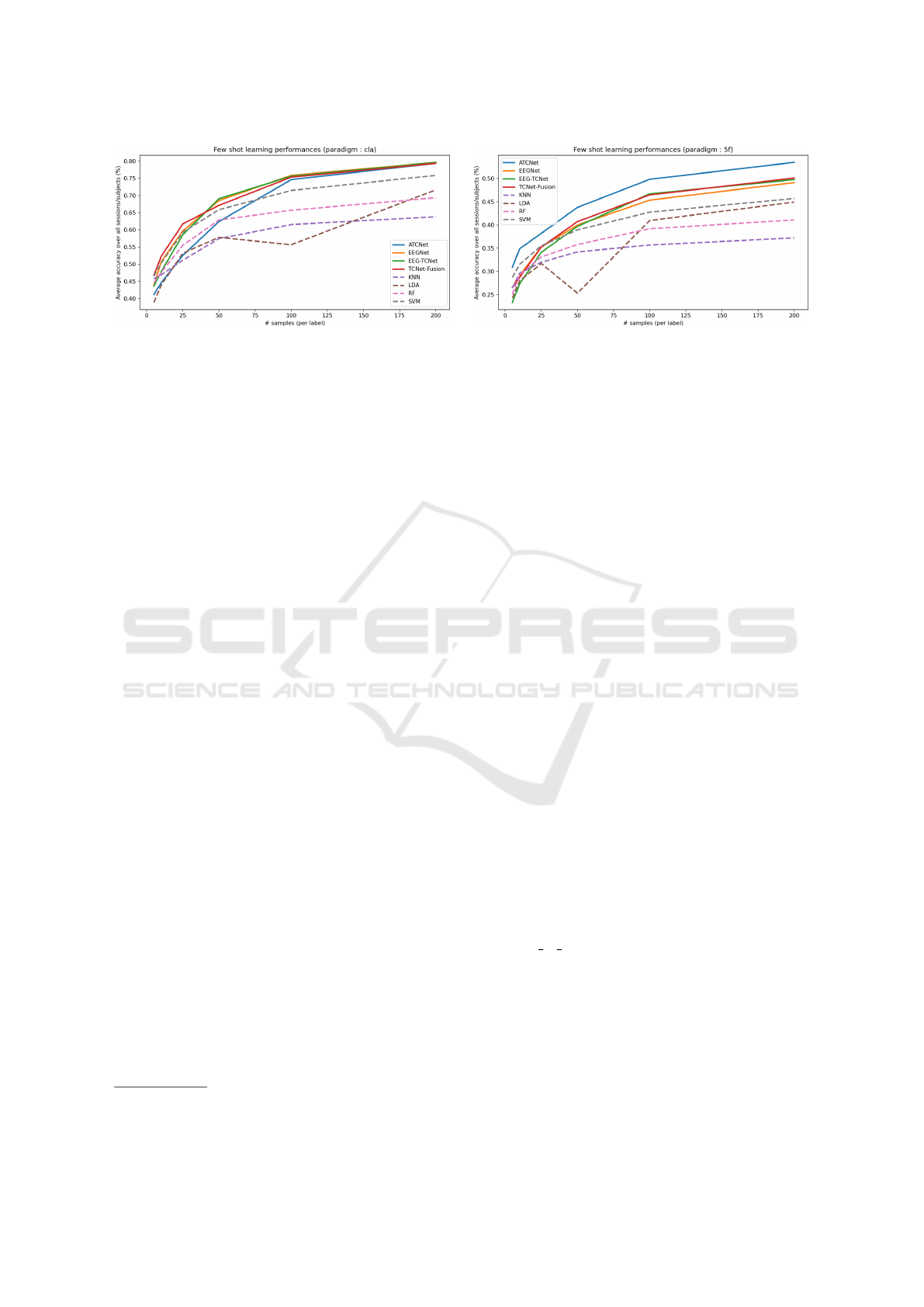
Figure 1: Average performance relative to the number of training samples on the CLA (left) and 5F (right) paradigms.
3 RESULTS AND DISCUSSION
This section presents the experimental results, along
with a detailed analysis and discussion of their impli-
cations for practical use cases. The results are orga-
nized into three distinct subsections, each providing
an in-depth analysis of a different experimental setup.
In addition to the standard performance metrics, a
time-based comparison is included for both training
and prediction times, allowing to assess the usabil-
ity of each model in real-time conditions. Finally, a
global discussion summarizes the findings and pro-
poses future research directions to further explore the
comparison between ML and DL approaches, as well
as their respective potentials.
3.1 Results in Low-Data Training
In the first experimental setup, models were trained on
data from a single subject session, with varying num-
bers of training samples. Table 4 shows the results
for each model alongside the corresponding number
of samples. Figure 1 provides a visual comparison
of performance between DL models (represented by
solid lines) and ML models (represented by dashed
lines) on the CLA and 5F paradigms.
It is important to note that the sample count in Ta-
ble 4 includes both the training and validation sets,
which were split in an 80-20 ratio, ensuring the same
number of samples per label in each set. Conse-
quently, in the first row for each paradigm, only 4
samples per label were used for training, with 1 sam-
ple per label used for validation. The “max” row cor-
responds to 80% of the entire session being used as
the training/validation sets, replicating the results of
Table 6 in the original paper (Kaya et al., 2018). Also,
note that the results for the SVM classifier are slightly
higher than those reported by Kaya et al., thanks to
3
The HaLT paradigm follows the same trend as the CLA
paradigm.
the use of raw signals instead of FTA features for
SVM, which has been found to slightly improve per-
formance.
The key observation is that even with a severely
limited number of training samples, some DL mod-
els outperform traditional ML classifiers, which
challenges the common assumption that ML mod-
els consistently perform better in low-data settings.
Nonetheless, the SVM classifier remains competitive,
outperforming most DL architectures when trained
with few samples.
Additionally, it is interesting to observe that, al-
though ATCNet remains one of the top performers
when all the training data is available, it performs
poorly with limited data, particularly on the CLA and
HaLT paradigms. This demonstrates that a state-of-
the-art model on one dataset is not necessarily the
best choice for other datasets or setups. As discussed
in Section 2.5, TCNet-Fusion provides a good bal-
ance between robustness and the number of param-
eters, making it a strong performer in low-resource
contexts.
To fully replicate the findings of Kaya et al.,
Figure 2 presents a BCI control analysis for the
three paradigms, comparing the ATCNet, TCNet-
Fusion, and SVM classifiers. In this analysis, sub-
jects are grouped into four performance categories:
low, intermediate-low, intermediate-high, and high
performers, based on model performance with all
training data available. The groups are equally di-
vided along a range from the chance level (100%
/ number of labels) to 100%. For example, in the
5F paradigm, the chance level is equal to 20% (=
100%/5), and the 4 groups respectively range from
20% to 40%, from 40% to 60%, from 60% to 80%,
and from 80% to 100%. The exact threshold values
for each group for the other paradigms are reported in
the Kaya et al. paper.
The main finding is that low-performing subjects
tend to remain low performers, even with DL mod-
els, while subjects in the other categories tend to shift
Comparison Between Machine Learning and Deep Learning on Multiple Motor Imagery Paradigms in a Low-Resource Context
709

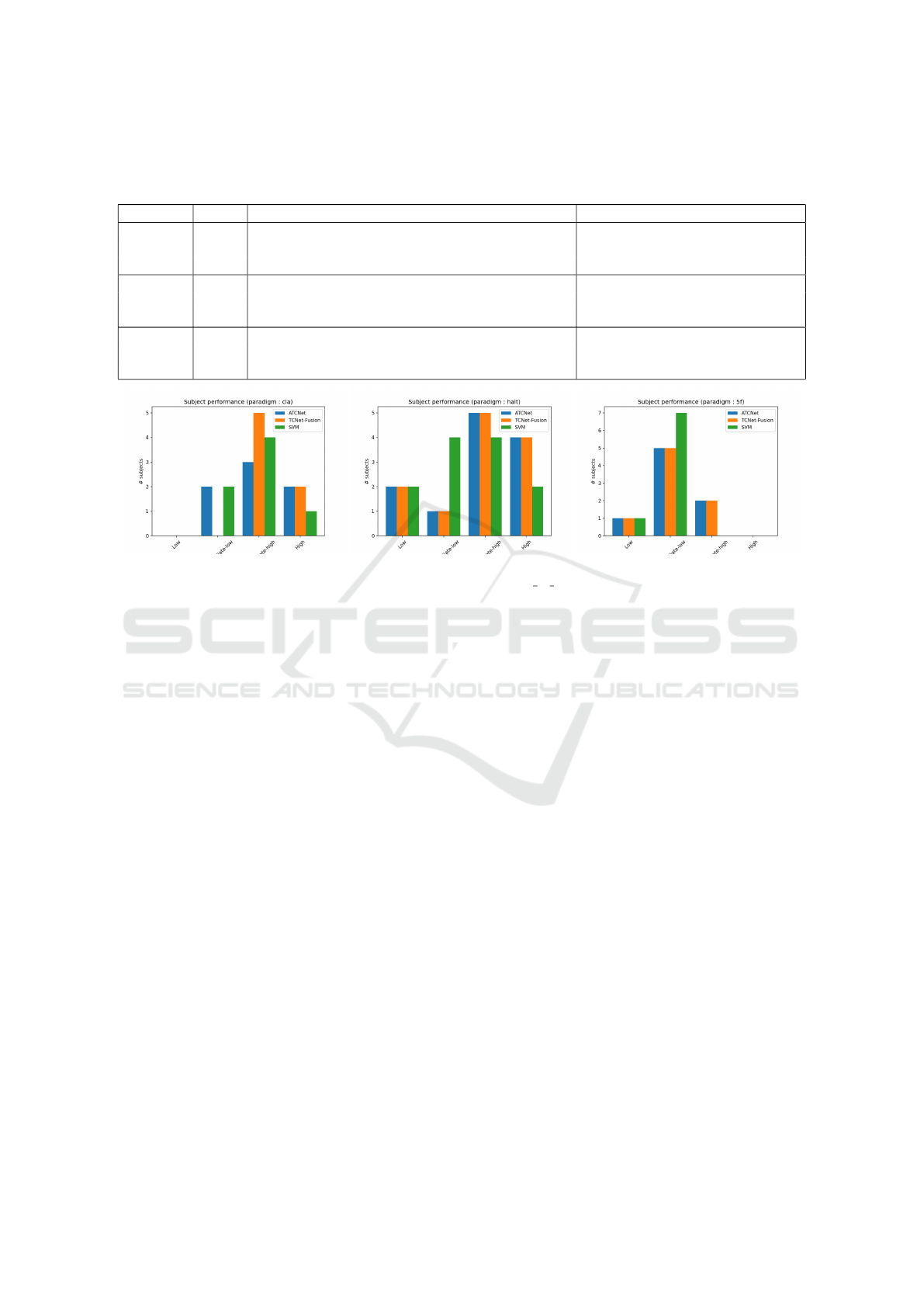
Table 4: Accuracy of each model on each paradigm, with varying number of training/validation data. The test set corresponds
to 20% of the entire session, while the training/validation samples (indicated in the second column) are randomly selected
from the remaining 80% of the session (cf. Section 2.3.).
Paradigm # data ATCNet TCNet-Fusion EEGTCNet EEGNet SVM RF LDA k-NN
CLA
15 41.2% 46.8% 43.6% 43.9% 46.6% 44.5% 38.9% 45.8%
30 44.6% 52.3% 47.8% 50.7% 50.3% 47.7% 43.9% 46.9%
max 79.4% 79.4% 79.6% 79.7% 75.9% 69.4% 71.6% 63.8%
HaLT
30 28.7% 36.2% 30.3% 34.1% 33.5% 29.6% 25.7% 30.1%
60 33.3% 43.0% 38.1% 41.8% 38.8% 35.2% 32.7% 33.6%
max 67.9% 68.6% 66.6% 67.2% 61.6% 52.5% 64.8% 47.7%
5F
25 30.9% 26.5% 23.3% 26.6% 28.7% 25.1% 24.2% 26.4%
50 34.9% 28.7% 27.3% 29.1% 31.5% 29.3% 28.0% 29.6%
max 53.5% 50.1% 49.8% 49.1% 45.7% 41.1% 44.9% 37.2%
Figure 2: BCI control performance for respectively the CLA (left), HaLT (middle) and 5F (right) paradigms. BCI controls are
defined as 4 equal groups ranging from chance level (defined as 1 / number of labels) to 1, as explained in the main text.
to higher performance groups, if replacing ML by
DL models. This is particularly evident in the CLA
paradigm, where all the intermediate-low performers
become intermediate-high performers if switching to
the TCNet-Fusion model.
3.2 Results with Multiple Sessions
Training
In the second experimental setup, models were
trained on all the sessions of a single subject. To en-
sure a fair comparison with the results from Table 4,
the test set comprises 20% of each session, guaran-
teeing that all sessions contribute equally to the final
performance, as they contain roughly the same num-
ber of trials. Table 5 presents the results obtained for
each model across each paradigm, averaged over all
the subjects.
These results demonstrate that, when more data
is available, DL models significantly outperform tra-
ditional ML models, particularly on more complex
MI paradigms such as HaLT and 5F. On the CLA
paradigm, which is easier to classify due to the con-
tralateral nature of the brain response in left/right
hand MI tasks, ML models remain competitive with
DL models. Interestingly, in the CLA paradigm, the
LDA classifier substantially benefits from the larger
dataset, with an average accuracy improvement of up
to 4.6%, as can be seen by comparing results from
the “max” row of Table 4 to the corresponding value
in Table 5. This represents the largest performance
increase among the models. In contrast, the SVM
and RF classifiers do not experience notable perfor-
mance gains from the inclusion of multiple sessions.
Meanwhile, DL models exhibit average performance
improvements of 3% on the CLA paradigm, 5% on
HaLT, and 1% on 5F. These findings are promising as
they suggest that models, particularly DL ones, can
leverage data from multiple sessions, despite the non-
stationary nature of EEG signals, leading to improved
performance.
3.3 Results with LOSO Training
In the third experimental setup known as LOSO train-
ing, models were trained on all the sessions from all
the subjects except for the left-out subject and were
evaluated on all the sessions from the left-out subject.
It is worth mentioning that these results can be fairly
compared to those in Tables 4 and 5, as all the ses-
sions equally contribute to the final results for a given
subject.
Table 6 illustrates the drop in performance when
compared to the other training setups, highlighting
the poor generalization of the models when applied
to new, unseen subjects. However, this is likely due
BIOSIGNALS 2025 - 18th International Conference on Bio-inspired Systems and Signal Processing
710

Table 5: Average accuracy for each model on each paradigm, if trained on multiple sessions from a single subject.
Paradigm ATCNet TCNet-Fusion EEGTCNet EEGNet SVM RF LDA k-NN
CLA 81.2 % 82.0 % 81.0 % 80.2 % 77.4 % 69.0 % 76.2 % 65.9 %
HaLT 70.5 % 72.0 % 69.8 % 69.2 % 64.6 % 53.5 % 67.4 % 48.5 %
5F 54.3 % 51.5 % 51.0 % 49.4 % 46.2 % 38.6 % 45.2 % 35.6 %
Table 6: Average accuracy for each model on each paradigm, if trained in a leave-one-subject out (LOSO) setting.
Paradigm ATCNet TCNet-Fusion EEGTCNet EEGNet SVM RF LDA k-NN
CLA 57.2 % 60.4 % 59.8 % 58.9 % 54.9 % 49.3 % 53.0 % 48.2 %
HaLT 54.0 % 56.5 % 53.7 % 52.8 % 50.5 % 39.2 % 48.2 % 35.6 %
5F 38.4 % 37.8 % 36.3 % 35.4 % 33.7 % 29.3 % 33.1 % 28.5 %
to the limited subject representation, as models were
trained on only 6 subjects for the CLA paradigm, 11
for the HaLT paradigm, and 7 for the 5F paradigm.
Based on the results reported by P
´
erez-Velasco et
al. in their LOSO training on 280 subjects (P
´
erez-
Velasco et al., 2022), a key future research area will
consist in reproducing these results while training
models on data from more subjects. The major chal-
lenge, however, will be to find such extensive data for
the different paradigms, especially for HaLT and 5F.
Despite the drop in performance, ranging from
15% (5F) to 20% (CLA) if compared against Table 4
that reported the training on all the available data, the
results are still 3% (5F) to 13% (HaLT) better than
those obtained when training/validating the models
with 10 samples per label. This suggests a promising
strategy for initializing models before applying them
to new subjects. Additionally, combining this strategy
with transfer learning has been shown to yield even
better results (Wu et al., 2022; Guetschel et al., 2022;
Li et al., 2023).
3.4 Time-Based Performance
This section presents the training and prediction times
for each model under the various experimental se-
tups. All experiments were conducted on the same
server equipped with an Intel Xeon W-2245 CPU and
a NVIDIA Quadro RTX 5000 GPU. Only the DL
models used the GPU. The visible memory of the
GPU was artificially restricted to 2GB of VRAM to
allow up to six parallel experiments. This setup was
manually tuned to avoid out-of-memory issues with-
out compromising performance.
3.4.1 Training Time
Figure 3 illustrates the average training time for each
model under different training conditions. The left
plot shows the average training time (y axis) as a func-
tion of the number of training samples (x axis) from
a single session, while the middle and right plots dis-
play the training time for models trained on all ses-
sions from a single subject and in a LOSO setup, re-
spectively. For DL models, the times are calculated
as the average time per epoch multiplied by the effec-
tive number of training epochs (i.e., after accounting
for the early-stopping patience). This explains why
models take longer to train on fewer samples, as they
require more epochs to converge. The training time
for the k-NN model is roughly equal to the data pro-
cessing time, as it only stores data points with their
label without any additional training mechanism.
One key observation is that only ML models can
be trained in real-time, while DL models require, on
average across all subjects and sessions, more than
15 seconds to converge during single-session train-
ing, around 1 minute for multiple sessions, and up
to half an hour for LOSO training
4
. These results
were obtained by training DL models using a rigorous
training and validation procedure, including early-
stopping criteria and intermediate checkpointing. In
a low-resource setup where a GPU is typically un-
available, some of these additional validation steps,
such as model checkpointing and convergence crite-
ria, may not be necessary. However, even after re-
moving redundant checkpoints and fixing the number
of epochs, experiments conducted on the CPU have
shown that DL models still require at least 5 seconds
to train for 50 epochs (which is insufficient for model
convergence), making them less competitive than ML
models in terms of training time performance.
On the other hand, when models are trained on
a large amount of data (e.g., multiple sessions or
LOSO), the training is not performed in real-time dur-
ing data acquisition. This suggests that if a larger
dataset is available, it may be more efficient to train
the model on all the data before the BCI device usage
session. As shown in Section 3.3, the results obtained
4
LOSO training includes around 15 training sessions,
depending on the left-out subject and on the MI paradigm.
Comparison Between Machine Learning and Deep Learning on Multiple Motor Imagery Paradigms in a Low-Resource Context
711

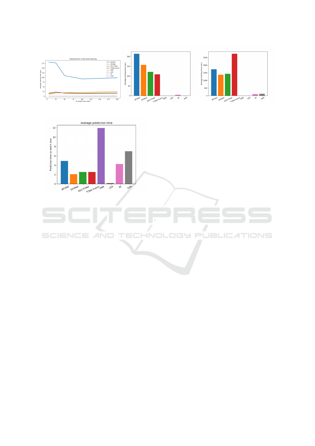
Figure 3: Average training time in a low-data context (left), with multiple sessions training (middle), and in LOSO training
(right).
Figure 4: Average prediction time on a batch of 64 samples.
in a LOSO context are better than those obtained with
fewer than approximately 25 samples per label, which
corresponds to 150 samples in the HaLT paradigm.
Furthermore, the LOSO setup used in this work in-
volves training on data from only up to 11 subjects
(or fewer, depending on the MI paradigm), which lim-
its inter-subject generalization. These results could
become even more significant if a larger number of
subjects were available, as demonstrated by P
´
erez-
Velasco et al., although this would significantly in-
crease the required training time (P
´
erez-Velasco et al.,
2022).
3.4.2 Prediction Time
Figure 4 depicts the average prediction time for each
model on a batch of 64 samples. LDA is by far
the fastest model, while most DL models, except
for ATCNet, are faster than RF and SVM models.
Nonetheless, all the models are usable in real-time
settings, as they can perform between 100 and 1,000
predictions per second. In the figure, DL models have
been executed on the GPU with additional optimiza-
tions offered by the TensorFlow framework. How-
ever, additional experiments conducted on the CPU
have shown that the prediction time of DL models is
less than doubled, making them still faster than the
SVM classifier.
The prediction time for the k-NN classifier has
been computed in the single-session setup on CPU.
In contrast to the other ML/DL models, it uses a
naive implementation that linearly depends on the
training data size, and its prediction time is there-
fore slower than the other experimental setups. How-
ever, more advanced implementations of the k-NN al-
gorithm may significantly reduce the prediction time,
making it usable in real-time, regardless of its number
of training samples (Johnson et al., 2019).
3.5 Discussion and Future Work
This section discusses the experimental results, focus-
ing on the impact of data availability, the differences
between intra- and cross-subject data, and the usabil-
ity of models in real-time conditions. Additionally,
potential directions for future research are proposed
to further explore the observations made in this study.
3.5.1 The Impact of Data
The primary objective of this work was to assess the
capability of DL models to perform well in low-data
contexts compared to traditional ML strategies. The
results in Table 4 demonstrate that DL models can
outperform ML approaches even with only 4 or 8
training samples per label. Additionally, Figure 1 il-
lustrates that as more data becomes available, the per-
formance gap between DL and ML models widens.
This difference is even more pronounced in complex
paradigms like HaLT and 5F, which is a significant
finding since these paradigms are less commonly an-
alyzed than the left/right hand (CLA) paradigm.
In addition to evaluating low-data setups, this
work also compared the ability of DL and ML models
to leverage multi-session data for training. This train-
ing setup provides more training data with greater
variability due to the non-stationary nature of EEG
signals. Despite this increased variability, DL models
were able to improve their average performance by
2% to 5%, depending on the paradigm. Conversely,
ML models generally did not benefit from this train-
ing setup, except for the LDA classifier in the CLA
BIOSIGNALS 2025 - 18th International Conference on Bio-inspired Systems and Signal Processing
712

paradigm. It is important to note that this finding is
preliminary, as the number of sessions per subject for
a given paradigm remains limited, as shown in Ta-
ble 1.
3.5.2 Intra vs. Cross-Subject Training
In addition to single- and multi-session training, we
compared the ability of ML and DL models to gen-
eralize to new, unseen subjects using a LOSO exper-
imental setup. It is important to note that our LOSO
experiments are based on a single dataset, which lim-
its the number of training subjects to between 6 and
11, depending on the paradigm. This limitation makes
it difficult to fairly compare intra-subject and cross-
subject training. However, despite the drop in perfor-
mance when transitioning from intra-subject to cross-
subject setups, the performance in the LOSO setup
remains higher than in low-data conditions.
Figure 1 suggests that LOSO results are roughly
equivalent to those obtained with 25 to 50 samples
per label, representing 75 to 150 samples for CLA and
125 to 250 for the 5F paradigm. Although this amount
of training and validation data might seem limited,
collecting such data requires a significant amount of
time and energy for the subject. For instance, in
the Kaya et al. data collection setting, where each
trial consists of 1 second of MI followed by a 2-
second break, collecting 75 samples would take ap-
proximately 225 seconds (around 4 minutes), while
collecting 250 samples would take about 750 seconds
(around 12 minutes).
These preliminary results are promising for appli-
cations where subjects need to calibrate the model be-
fore use, particularly when combined with other ad-
vanced modern strategies, which will be discussed in
the following sections.
3.5.3 ML vs. DL in Real-Time Setups
The last comparison in this work is a time-based
benchmark of both training and prediction times. It
is evident that only ML models are capable of being
trained in real-time conditions, which corresponds to
the situation where the model must be trained during
the data acquisition process.
Nonetheless, small DL models can still be trained
within seconds, making it feasible to train them dur-
ing a BCI session. This enables the possibility of
training both ML and DL models in parallel: The
ML model could be used to provide live feedback
during the calibration phase, and the DL model to
deliver higher-quality predictions during the remain-
der of the session. Such a strategy can be applied to
any BCI application requiring an initial calibration of
the model, such as neuro-gaming or orthosis control.
However, training DL models in low-resource con-
ditions requires special attention and careful design
choices to limit computational demands and to detect
convergence to avoid overfitting.
Finally, as discussed in Section 4, both ML and
DL models can perform predictions on a CPU in 5 to
10 milliseconds, which is more than adequate for BCI
device control or real-time monitoring.
3.5.4 Future Work
This section outlines several potential research areas
that could be explored to either further compare mod-
els on MI decoding in different scenarios or to inves-
tigate the potential benefits of each approach high-
lighted in this study. The objective is to propose ro-
bust comparison and evaluation strategies that assess
performance under practical conditions, making them
valuable approaches for MI-BCI applications.
Few-Shot Multi-Session Training. In this work, the
multi-session training setup was explored to com-
pare the ability of ML and DL approaches to ben-
efit from larger amounts of data from a single sub-
ject. A more practical strategy would be to train
models on limited data from each session, sim-
ulating the collection of small datasets at the be-
ginning of each session. This approach could help
evaluate the impact of data variability due to the
non-stationary nature of EEG signals, when us-
ing limited data from each session, which more
closely mirrors real-world scenarios.
Multi-Task Training. In this work, each MI
paradigm was handled separately to evaluate the
impact of different motor imageries on model
performance. However, this has been shown that
DL models can benefit from having more data
from the same subject. A promising research
direction would be to train models on all sessions
from a single subject by combining data from all
MI paradigms. The challenge in this approach
would be to manage label imbalance, as not
all MI tasks are equally represented, especially
considering that the left/right hand tasks appear
in both the CLA and HaLT paradigms.
Few-Shot Transfer Learning. This study primarily
focused on few-shot learning strategies, given that
traditional ML models are typically not designed
for fine-tuning. However, as highlighted by N.
Mammone, few-shot cross-task transfer learning
is a promising approach for training models on
new MI tasks with limited data from the target
task (Mammone et al., 2024). Additionally, few-
shot cross-subject transfer learning has demon-
Comparison Between Machine Learning and Deep Learning on Multiple Motor Imagery Paradigms in a Low-Resource Context
713

strated potential for generalizing to new subjects
with only a small amount of data from the left-
out subject (Wu et al., 2022; Li et al., 2023).
These strategies represent promising research ar-
eas to extend both the multi-task training setup de-
scribed above and the LOSO setup studied in this
work.
Semi-Supervised Learning. In this study, the few-
shot learning strategy was used to simulate the
model calibration phase at the beginning of the
MI-BCI session, utilizing only a small amount of
data while discarding the rest. During this calibra-
tion phase, the subject performs predefined mo-
tor imageries at specific times, allowing the corre-
sponding EEG data to be mapped to expected la-
bels. However, once the calibration phase is com-
plete, the model is expected to perform predic-
tions on data without label mapping, preventing
further model training on these new data. Semi-
supervised learning presents a promising research
direction that could leverage these additional un-
labeled data to further calibrate and improve the
model, as suggested by Yu et al. in the context
of sensor-based Human Activity Recognition (Yu
et al., 2023).
4 CONCLUSION
This study presents a comprehensive and robust com-
parison between traditional ML and DL strategies
across multiple MI classification paradigms. In ad-
dition, various training and evaluation setups were in-
troduced to compare the models under different con-
ditions, highlighting the strengths and limitations of
each technique. A time-based benchmark was also
conducted to evaluate the usability of both ML and
DL models in real-time conditions. The results indi-
cate that, despite the common belief that DL models
require large amounts of data to achieve high-quality
results, they can still compete with or even outperform
ML models in low-data conditions. Moreover, DL
models demonstrated their ability to benefit signifi-
cantly from larger datasets, in contrast to ML strate-
gies. Lastly, while both ML and DL models showed
potential for real-time application, thanks to a predic-
tion time between 1 and 10 milliseconds, only ML
models were viable candidates for training during live
data acquisition. These findings open new research
questions and future work areas that are related to
few-shot multi-session training, multi-task training,
few-shot transfer learning, and semi-supervised learn-
ing.
ACKNOWLEDGEMENTS
Quentin Langlois is funded by the Walloon Region
through a F.R.S.-FNRS FRIA (Fund for Research
training in Industry and Agriculture) grant.
REFERENCES
Alkoby, O., Abu-Rmileh, A., Shriki, O., and Todder, D.
(2017). Can we predict who will respond to neuro-
feedback? A review of the inefficacy problem and
existing predictors for successful eeg neurofeedback
learning. Neuroscience, 378.
Altaheri, H., Muhammad, G., and Alsulaiman, M. (2023).
Physics-informed attention temporal convolutional
network for EEG-based motor imagery classifica-
tion. IEEE Transactions on Industrial Informatics,
19(2):2249–2258.
Angulo-Sherman, I. and Guti
´
errez, D. (2014). Effect of
different feedback modalities in the performance of
brain-computer interfaces. In CONIELECOMP 2014
- 24th International Conference on Electronics, Com-
munications and Computers, pages 14–21.
Breiman, L. (2001). Random forests. Machine Learning,
45:5–32.
Chen, X., Teng, X., Chen, H., Pan, Y., and Geyer,
P. (2024). Toward reliable signals decoding for
electroencephalogram: A benchmark study to EEG-
NeX. Biomedical Signal Processing and Control,
87:105475.
Chollet, F. et al. (2015). Keras. https://keras.io.
Gramfort, A., Strohmeier, D., Haueisen, J., H
¨
am
¨
al
¨
ainen,
M., and Kowalski, M. (2013). Time-frequency mixed-
norm estimates: Sparse M/EEG imaging with non-
stationary source activations. NeuroImage, 70.
Guetschel, P., Papadopoulo, T., and Tangermann, M.
(2022). Embedding neurophysiological signals. In
2022 IEEE International Conference on Metrology for
Extended Reality, Artificial Intelligence and Neural
Engineering (MetroXRAINE), pages 169–174.
Hearst, M., Dumais, S., Osuna, E., Platt, J., and Scholkopf,
B. (1998). Support vector machines. IEEE Intelligent
Systems and their Applications, 13(4):18–28.
Ingolfsson, T., Hersche, M., Wang, X., Kobayashi, N., Cav-
igelli, L., and Benini, L. (2020). EEG-TCNet: An ac-
curate temporal convolutional network for embedded
motor-imagery brain-machine interfaces.
Isa, N., Amir, A., Ilyas, M., and Razalli, M. (2019). Mo-
tor imagery classification in brain computer interface
(BCI) based on EEG signal by using machine learn-
ing technique. Bulletin of Electrical Engineering and
Informatics, 8:269–275.
Johnson, J., Douze, M., and J
´
egou, H. (2019). Billion-scale
similarity search with GPUs. IEEE Transactions on
Big Data, 7(3):535–547.
Kaya, M., Binli, M., Ozbay, E., Yanar, H., and Mishchenko,
Y. (2018). A large electroencephalographic motor im-
BIOSIGNALS 2025 - 18th International Conference on Bio-inspired Systems and Signal Processing
714

agery dataset for electroencephalographic brain com-
puter interfaces. Scientific Data, 5:180211.
Kingma, D. and Ba, J. (2014). Adam: A method for
stochastic optimization. International Conference on
Learning Representations.
Lawhern, V., Solon, A., Waytowich, N., Gordon, S., Hung,
C., and Lance, B. (2016). EEGNet: A compact con-
volutional network for eeg-based brain-computer in-
terfaces. Journal of Neural Engineering, 15.
Lebedev, M. A. and Nicolelis, M. A. L. (2017). Brain-
machine interfaces: From basic science to neuro-
prostheses and neurorehabilitation. Physiological Re-
views, 97(2):767–837. PMID: 28275048.
LeCun, Y., Bengio, Y., and Hinton, G. (2015). Deep learn-
ing. Nature, 521:436–44.
Li, A., Wang, Z., Zhao, X., Xu, T., Zhou, T., and Hu, H.
(2023). MDTL: A novel and model-agnostic trans-
fer learning strategy for cross-subject motor imagery
BCI. IEEE Transactions on Neural Systems and Re-
habilitation Engineering, PP:1–1.
Mammone, N., Ieracitano, C., Spataro, R., Guger, C.,
Cho, W., and Morabito, F. (2024). A few-shot trans-
fer learning approach for motion intention decoding
from electroencephalographic signals. International
Journal of Neural Systems, 34(02):2350068. PMID:
38073546.
Mishchenko, Y., Kaya, M., Ozbay, E., and Yanar, H.
(2019). Developing a three- to six-state EEG-based
brain–computer interface for a virtual robotic manip-
ulator control. IEEE Transactions on Biomedical En-
gineering, 66(4):977–987.
Mulder, T. (2007). Motor imagery and action observation:
Cognitive tools for rehabilitation. Journal of neural
transmission (Vienna, Austria : 1996), 114:1265–78.
Musallam, Y., AlFassam, N., Muhammad, G., Amin, S.,
Alsulaiman, M., Abdul, W., Altaheri, H., Bencherif,
M., and Algabri, M. (2021). Electroencephalography-
based motor imagery classification using temporal
convolutional network fusion. Biomedical Signal Pro-
cessing and Control, 69:102826.
P
´
erez-Velasco, S., Santamar
´
ıa-V
´
azquez, E., Mart
´
ınez-
Cagigal, V., Marcos Mart
´
ınez, D., and Hornero, R.
(2022). EEGSym: Overcoming inter-subject variabil-
ity in motor imagery based bcis with deep learning.
IEEE transactions on neural systems and rehabilita-
tion engineering : a publication of the IEEE Engi-
neering in Medicine and Biology Society, PP.
Tangermann, M., M
¨
uller, K.-R., Aertsen, A., Birbaumer,
N., Braun, C., Brunner, C., Leeb, R., Mehring, C.,
Miller, K., M
¨
uller-Putz, G., Nolte, G., Pfurtscheller,
G., Preissl, H., Schalk, G., Schl
¨
ogl, A., Vidaurre, C.,
Waldert, S., and Blankertz, B. (2012). Review of the
BCI competition IV. Frontiers in neuroscience, 6:55.
Tibrewal, N., Leeuwis, N., and Alimardani, M. (2022).
Classification of motor imagery EEG using deep
learning increases performance in inefficient BCI
users. PLOS ONE, 17:e0268880.
Vaswani, A., Shazeer, N., Parmar, N., Uszkoreit, J., Jones,
L., Gomez, A. N., Kaiser, L. u., and Polosukhin,
I. (2017). Attention is all you need. In Guyon,
I., Luxburg, U. V., Bengio, S., Wallach, H., Fer-
gus, R., Vishwanathan, S., and Garnett, R., editors,
Advances in Neural Information Processing Systems,
volume 30. Curran Associates, Inc.
Wu, D., Jiang, X., and Peng, R. (2022). Transfer learning
for motor imagery based brain–computer interfaces:
A tutorial. Neural Networks, 153:235–253.
Yu, H., Chen, Z., Zhang, X., Chen, X., Zhuang, F., Xiong,
H., and Cheng, X. (2023). FedHAR: Semi-supervised
online learning for personalized federated human ac-
tivity recognition. IEEE Transactions on Mobile Com-
puting, 22(6):3318–3332.
Comparison Between Machine Learning and Deep Learning on Multiple Motor Imagery Paradigms in a Low-Resource Context
715