Real-Time Digital Twin for Construction Vehicle Stability Assessment

and Visualization with Improved Front-Loader Payload Estimation

eo Tuerlinckx

1 a

, Sam Weckx

1 b

, Steven Robyns

1 c

and Jeroen D. M. De Kooning

2,3 d

MotionS Corelab, FlandersMake, 133 Oude Diestersebaan, 3920 Lommel, Belgium

Department of Electromechanical, Systems and Metal Engineering, Faculty of Engineering and Architecture,

Ghent University, Belgium

{theo.tuerlinckx, sam.weckx, steven.robyns}@ﬂandersmake.be, jeroen.dekooning@ugent.be

Keywords:

Construction Vehicle, Digital Twin, Stability Assessment, Stability Visualization, Payload Estimation Method,

Multibody Modelling.

Abstract:

The stability assessment of construction vehicles, which are part of a constantly growing market, is of a high

importance for safety and working efﬁciency. For such vehicles, the stability is mainly impacted by the carried

payload. In this paper, a state of the art payload estimation method, based on simpliﬁed motion equations, is

further improved by coupling it with accurate real-time multibody modelling. An example, that allows to

reduce the important impact of joints damping on the payload estimation method, is developed and validated

in this paper. A reduction of the payload estimation moving window root mean square error from 12.8% to

2.9% is obtained. Finally, the tractor multibody digital-twin is integrated in a real-time system on a physical

setup, allowing to process the signals of the tractor and provide an easy to interpret visualization of the vehicle

stability to the operator.

1 INTRODUCTION

The market of construction vehicles, such as bull-

dozers, excavators, tractors with front-loader, etc, is

constantly growing because of the increase of con-

struction activities due the expansion of the human-

ity (MarkwideResearch, 2024). This trend is also

followed by an integration of Advanced Driver As-

sistance Systems (ADAS) to improve the safety and

efﬁciency of those vehicles (AlliedMarketResearch,

2024). The main study concern in this paper is the sta-

bility of construction vehicles. Going towards more

efﬁcient construction means moving higher payloads

at higher speeds. This payload, whose value and ex-

act position are often unknown by the operator, can

lead to instability of the vehicle and even rollover

(Zhu et al., 2021). Additionally to the payload value

and position, the vehicle suspension plays an impor-

tant role for the vehicle stability while it is moving

(Cordos¸ and TodoruT¸ , 2019). However, this research

https://orcid.org/0000-0001-9780-0714

https://orcid.org/0000-0001-6983-495X

https://orcid.org/0000-0001-5898-7061

https://orcid.org/0000-0002-0358-4350

is only focusing on the payload estimation impact on

vehicle stability and not the suspension system.

A lot of research already focused on the anal-

ysis of stability behaviour in construction vehicles.

(Mitrev and Marinkovi

c, 2019) is performing a full

numerical study for the stability of an excavator, in-

cluding the tire suspensions, while (Edwards et al.,

2019) focuses on the risk of overturning. However,

both are assuming a known payload. (Lysych, 2020)

is using SolidWorks to study the dynamics of a trac-

tor, including working tools at the front and rear of

the vehicle, but without taking into account the move-

ment of those tools. (Baker and Guzzomi, 2013) is

analysing the stability of a tractor on a slope by in-

cluding the effect of the front axle-wheel mass, under-

lining the important impact of it on the overall Center

Of Gravity (COG) position but without including the

impact of the front-loader and its payload. It can be

seen that therefore most of the research about con-

struction vehicle stability assumes a know payload or

are not including the dynamics of the front-loader.

By looking at the state of the art in estimating

payload, the research of (Ferlibas and Ghabcheloo,

2021), that will be further analysed in this paper,

presents a novel approach for dynamic payload esti-

266

Tuerlinckx, T., Weckx, S., Robyns, S. and M. De Kooning, J. D.

Real-Time Digital Twin for Construction Vehicle Stability Assessment and Visualization with Improved Front-Loader Payload Estimation.

DOI: 10.5220/0013080500003941

Paper published under CC license (CC BY-NC-ND 4.0)

In Proceedings of the 11th International Conference on Vehicle Technology and Intelligent Transport Systems (VEHITS 2025), pages 266-277

ISBN: 978-989-758-745-0; ISSN: 2184-495X

mation on an excavator without including joints fric-

tion and damping. (Bennett et al., 2014) use a multi-

body model to study the impact of static and dy-

namic behaviour of an excavator on payload estima-

tion methods in simulation. Moreover, a state esti-

mator (Ishihara et al., 2021) or neural network (Huo

et al., 2023) can also be used to estimate payload of

construction vehicles. On the other side, other re-

searchers are focusing on accurate and complex mod-

eling of construction vehicles with multibody model-

ing (Pavlov and Dacova, 2021) or the ﬁnite element

method (Gralak and Walu

s, 2024), but also assume a

known payload.

This paper aims to bridge the gap between sim-

pliﬁed payload estimation methods and the accuracy

of multibody modeling. It focuses on developing a

digital twin of a tractor using Simscape Multibody,

including the hydraulic front-loader and suspension

systems. The digital twin is deﬁned as a virtual replica

that acts and behaves like its physical counterpart,

with automated data transfer between the physical

system and the virtual model. The multibody model

is coupled with an adapted payload estimation method

and validated through experimental tests on a physi-

cal tractor setup. The research highlights the potential

to improve or analyze the stability of construction ve-

hicles by coupling multibody modeling with payload

estimation methods. It also presents an improved pay-

load estimation method that is robust to joint damp-

ing, which can signiﬁcantly impact construction ve-

hicles. Finally, the digital twin is integrated into a

real-time system on the physical setup, allowing for

signal processing and 3D visualization of vehicle sta-

bility for the operator.

The paper is structured as follows. The second

section describes the theory, models, and methods

for tractor multibody modeling, payload estimation,

and stability assessment. Section 3 details experi-

ments validating these methods with ﬁeld measure-

ments. Finally, the Section 4 discusses the results and

Section 5 provides a summary and outlook.

2 THEORY, MODELS AND

METHODS

In order to validate the improvement on construction

vehicle stability assessment and visualization, a rele-

vant industrial case of a construction vehicle is used.

A New Holland T7.175 SideWinder II tractor with a

Still front loader 770TL is modelled as a multi-body

model and used as real physical setup for data collec-

tion. The physical setup is also used to gather sig-

nals that will be used as input for the model such

as the front-loader positions or hydraulic pressures.

The tractor has a front-loader actuated by an hydraulic

system with different possibilities of working imple-

ments (i.e. a bucket or a fork). The suspension system

is made of a front-axle TerraGlide suspension devel-

oped by New Holland.

In order to assess the stability of the tractor, ﬁrstly,

an estimation of the front-loader payload is calcu-

lated. Secondly, the tractor center of gravity is com-

puted based on the weight distribution. Thirdly, the

tractor stability is discussed, taking into account the

inﬂuence of the tractor pitch. Finally the visualization

of the tractor stability to the vehicle operator and the

overall real-time implementation architecture are de-

picted. The following subsections describe the phys-

ical and simulated model and the real-time methods

and architecture used for front-loader payload estima-

tion and stability assessment and visualization.

2.1 Physical Setup

The T7.175 tractor physical setup can be seen in Fig-

ure (1). The setup is made of two main subsystems :

the front-loader hydraulic system and the suspensions

system, which are described in the section below.

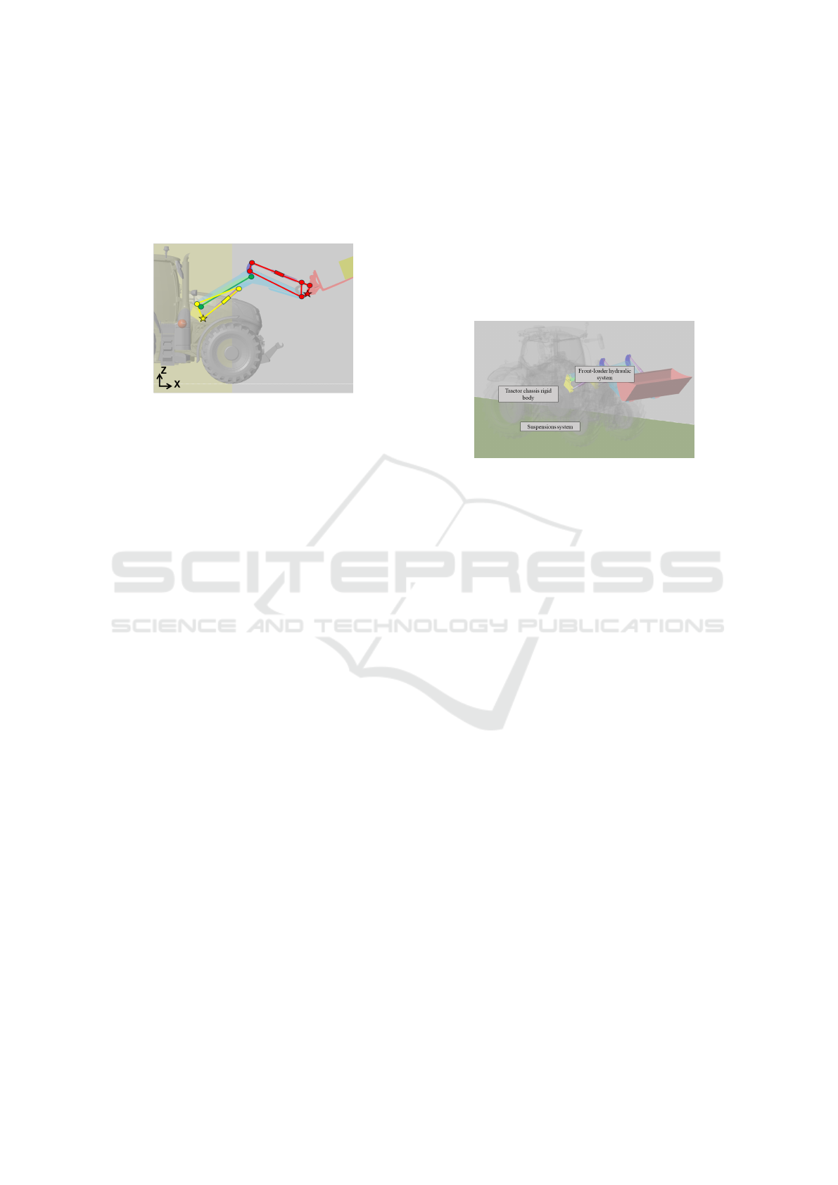
Figure 1: Tractor physical setup.

2.1.1 Front-Loader Hydraulic System

The front-loader has two main degrees of freedom

(DOF). The main arm (blue part in Figure (2)) rotates

along the Y-axis relative to the tractor chassis (see yel-

low star in Figure (2)), and the implement (red part)

rotates along the Y-axis relative to the arm tip (see

red star). A hydraulic pump, driven by the tractor’s

engine, provides pressure and ﬂow to the hydraulic

cylinders (schematized as the yellow and red rectan-

gle), which are part of a kinematic closed loop. This

means the movements of the rotational DOFs are di-

rectly linked to the translational motions of the hy-

draulic cylinders.

Hydraulic ﬂow is controlled by a lever, and

the pump adjusts pressure based on the payload to

achieve the desired movement. A system of valves

maintains pressure in the hydraulic cylinders when

Real-Time Digital Twin for Construction Vehicle Stability Assessment and Visualization with Improved Front-Loader Payload Estimation

267

the front-loader is stationary, allowing it to carry

heavy loads without consuming power. Additionally,

a payload stabilization system (green bar) ensures the

implement remains stable when the main arm moves,

preventing the payload from falling off by linking the

two DOF’s.

Figure 2: Front-loader degrees of freedom.

2.1.2 Suspensions System

The main suspension behavior of a tractor comes

from the tire radial stiffness and damping that makes

the connection between the chassis and the ground

(Cuong et al., 2013). Additionally to this, a Ter-

raGlide front-axle suspension system has been de-

veloped by NewHolland (New Holland Agriculture,

2024).

2.1.3 Sensors

The setup includes multiple sensors and an Industrial

PC for processing sensor signals. Key components

are:

• Leopard Imaging GMSL AR0231 camera: Es-

timates angles of the front-loader’s main arm

and implement using low cost vision methods

(Robyns et al., 2024).

• PU501E pressure sensors: Measure pressure in

both chambers of the hydraulic cylinders.

• Xsense MTi-30 Inertial Measurement Units

(IMU): Provide roll and pitch measurements, with

one unit on the chassis below the cabin and an-

other on the front-axle below the suspension pivot

point.

2.2 Simulation Multi-Body Model

A digital-twin of the tractor physical model is built

in order to develop and validate the front-loader pay-

load estimation and stability assessment as well as the

visualization methods. The simulation model is im-

plemented in the MATLAB environment, using the

Simscape Multibody Library for simulating the trac-

tor multi-body model while Simulink is used for post

and pre-processing of the signals (e.g. computation

of the hydraulic cylinder forces, payload estimation

method, ...).

The Figure (3) shows the 3D visualization of the

tractor Simscape Multibody model. The main chas-

sis rigid body is imported as one CAD ﬁle while the

two other subsystems, the suspensions and the front-

loader hydraulics, are explained in more details in the

following subsections.

Figure 3: 3D visualization of the Tractor Simscape Multi-

body model with underlined subsystems.

2.2.1 Front-Loader Hydraulic System

The front-loader hydraulic system has two closed-

loops for the main arm and implement on both sides,

but only the right side is actuated in the simulation

for simplicity. As the main arm and implement are

modeled as rigid bodies, the left side of the model

will follow the same movement. The kinematic close-

loops are modeled in Simscape Multibody using pris-

matic and revolute joints, with one joint actuated by

input and others automatically computed. The physi-

cal setup uses prismatic joints for actuation, while the

simulation uses the revolute joints, demonstrating the

beneﬁts of a low-cost camera sensor for their position

measurement (Robyns et al., 2024).

The front-loader payload estimation method re-

quires the computation or measurement of torque in

the DOF joints. In a Simscape Multibody model,

this torque can be directly extracted from the revolute

joints and is based on component inertias, payload,

and front-loader movement. A virtual payload can

be simulated by adding a variable mass component

to the implement. However, in real industrial applica-

tions where the payload is unknown, the method must

compute the joint’s torque using regular sensors with

the following approach.

Knowing the pressure in the hydraulic cylinders,

their forces can be computed as the difference in force

between the two chambers:

F = F

− F

(1)

VEHITS 2025 - 11th International Conference on Vehicle Technology and Intelligent Transport Systems

268

Figure 4: Hydraulic cylinder schematic.

with:

F = A · P (2)

With P the hydraulic pressure in Pascal and A the

chamber bore area in m

(see Figure (4)):

· D

(3)

and



− D

Rod



(4)

Regarding the hydraulic pressure, this one is mea-

sured before the chambers. In order to account for the

pressure loss in the hydraulic circuit between the sen-

sors and the chambers (i.e. junction, bend, etc), the

pressure measurement is multiplied by an efﬁciency

factor:

P = P

· η

(5)

Once the hydraulic cylinder force is computed, it

can be applied as an input force to the cylinder pris-

matic joint of the model. The Simscape Multibody

model, by multiplying those forces with the cylinder

jacobians, can directly extract the torque in the DOF

revolute joints, knowing the hydraulic cylinder pres-

sure and corresponding DOF’s positions. The torques

are computed with a multibody model with compo-

nents with an inﬁnitely small density and no payload

in the implement as the hydraulic pressure measure-

ment on the physical setup already includes those el-

ement effects.

2.2.2 Suspensions System

This subsystem is modelled and validated using the

IMU’s measurement with the tractor at standstill.

However the rolling vehicle with acceleration and de-

celeration is not yet modelled. Therefore, the study of

the impact of the suspension subsystem on the vehicle

stability is not further investigated here.

2.2.3 Solver and Parameters Value

Simscape Multibody uses a ﬁxed time step to solve

the equations of motion for the mechanical system.

Simulink systems (i.e. computation of the hydraulic

cylinder force, payload estimation, etc.) use a ﬁxed

step solver (Bogacki–Shampine) for third-order ordi-

nary differential equations. The time step allows real-

time simulation, enabling integration into a physical

setup for stability assessment and smooth visualiza-

tion.

Finally, the overall parameter values of the multi-

body model are summarized in the Table (1).

Table 1: Tractor multibody-model parameters.

Parameters Units Value

ρ kg/m

5500

Tractor

kg 6000

M kg 10

Piston,Arm

m 0.1475

PistonRod,Arm

m 0.0381

P,Arm

% 0.58

Piston,Implement

m 0.1079

PistonRod,Implement

m 0.0165

P,Implement

% 0.69

m 2.97

arm

kgm

780.8

arm

kg 1320

rad 0.23

m 1.42

m 2.85

imp

kgm

34.59

imp

kg 272.7

rad 0.2663

m 0.4723

HC,Arm

N/(m/s) 3.9e+05

HC,Implement

N/(m/s) 1.15e+05

T s

Simscape

s 1e-03

T s

Simulink

s 1e-03

2.3 Front-Loader Payload Estimation

The front-loader payload estimation used within this

paper is based on (Ferlibas and Ghabcheloo, 2021)

and schematized in Figure (5). The front-loader can

be considered as a three-revolute joint manipulator in

the vertical plane with the tractor pitch, the main arm

and the implement joint. The dynamic torque equa-

tions of that manipulator are rewritten in a decoupled

form as the linear combination of dynamic gravita-

tional parameters and functions of joint angles, ve-

locities, and accelerations. A measurement campaign

without payload on the physical setup can then be per-

formed to measure the joint torques with their corre-

sponding joint position and speed. A least squares es-

timation can then be used to identify the gravitational

parameters for a joint conﬁguration without payload.

Therefore, when performing a measurement with pay-

load, the relation between the actual with-load torque

can be made with the estimated without-load torque

using the gravitational parameters. From this rela-

Real-Time Digital Twin for Construction Vehicle Stability Assessment and Visualization with Improved Front-Loader Payload Estimation

269

tion, an estimation of the payload can be computed

(Ferlibas and Ghabcheloo, 2021). The summarized

method is now presented in more details.

As the front-loader can be considered as a three-

revolute joint manipulator in the vertical plane, the

dynamics can be described with the following equa-

tion (Ferlibas and Ghabcheloo, 2021):

τ = D(Θ)

Θ +C(Θ,

Θ) + G(Θ) (6)

With:

• τ: the joint torque vector

• Θ: the vector of joint angles

• D(Θ): the inertia matrix

• C(Θ,

Θ): the vector of Coriolis and centrifugal

terms

• G(Θ): the gravity torque vector

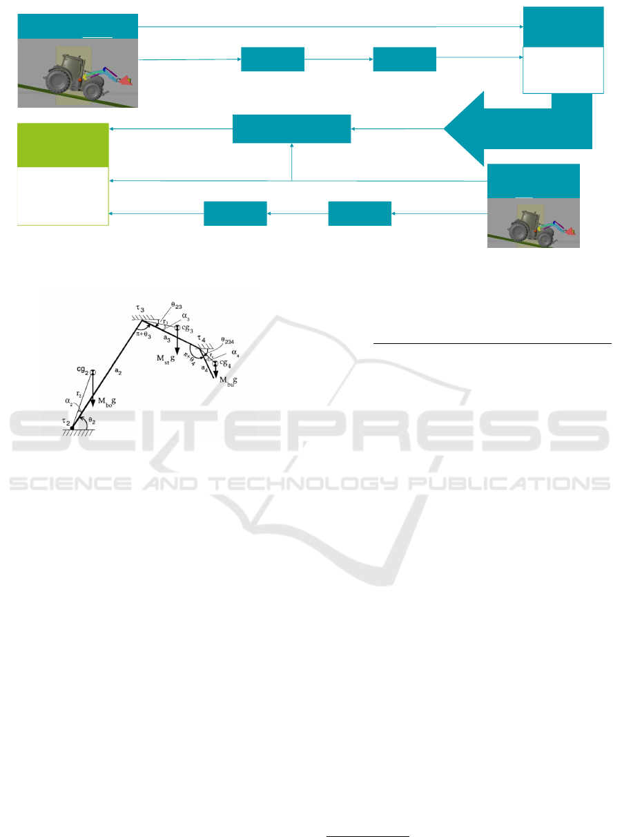
And with the corresponding schematic diagram in

Figure (6) where θ

is the pitch angle, θ

the arm

angle and θ

234

the implement angle.

As explained above, the torque equation (6) can

be rewritten in a decoupled form as the linear combi-

nation of dynamic gravitational parameters, π, and a

matrix Y function of joint angles, velocities, and ac-

celerations:

τ = Y (Θ,

Θ,

Θ)π (7)

By neglecting the friction and damping in the

joints, the linear torque equations can be obtained us-

ing Euler-Lagrange method (Ferlibas and Ghabche-

loo, 2021):

τ4 = (I

imp

+ M

imp

)

234

+ M

imp

[

cos(θ

+ α

) +

sin(θ

+ α

)]

+ M

imp

[

cos(θ

+ α

) +

sin(θ

+ α

)]

+ M

imp

cos(θ

234

+ α4)

τ3 = τ4 + (I

arm

+ M

arm

+ M

imp

)

+ M

imp

[

cos(θ

) +

sin(θ

)]

+ M

imp

[

234

(θ

+ α

) −

234

sin(θ

+ α

)]

+ M

arm

[

(θ

+ α

) +

sin(θ

+ α

)]

+ M

imp

cos(θ

) + M

arm

cos(θ

+ α

)

(8)

With:

• I

arm

imp

: the moments of inertia of the main arm

and implement respectively

• M

arm

imp

: the masses of the main arm and im-

plement respectively

• a

: the linear distance between the pitch joint and

the arm joint

• a

: the linear distance between the arm joint and

the implement joint, also called the arm length in

that paper.

• α,r: the polar coordinates of the center of gravity

of the arm

and the implement

Note that the torque equation of the pitch τ

has

not been written as the pitch torque is not measured

on the physical setup and therefore cannot be used.

2.3.1 Dynamic Estimation of the Payload

Now that the torque equations have been described,

they can be rewritten in the matrix form of (7), (Fer-

libas and Ghabcheloo, 2021):







0 y

0 0

0 y















(9)

with τ

= τ

− τ

and:

234

= a

cos(θ

) + a

sin(θ

) + a

cos(θ

)

+ a

sin(θ

) + gcos(θ

234

)

= − a

sin(θ

) + a

cos(θ

) − a

sin(θ

)

+ a

cos(θ

) − gsin(θ

234

)

= a

234

cos(θ

) − a

234

sin(θ

)

= − a

234

sin(θ

) − a

234

cos(θ

)

= a

cos(θ

) + a

sin(θ

) + gcos(θ

)

= − a

sin(θ

) + a

cos(θ

) − gsin(θ

)

(10)

Using that set of linearized equations, the gravita-

tional parameters π can be estimated using the Least

Squares Estimation method with a set of measure-

ments (without payload) of the joints torque without

payload τ and joints position θ. As the joints velocity

θ and acceleration

θ are not measured on the physical

setup, their values are simpliﬁed as the derivatives of

the position.

Thereafter, when adding a payload M

in the im-

plement, assuming that the implement center of grav-

ity is ﬁxed and does not change depending on the

variable load weight in the implement (Ferlibas and

Ghabcheloo, 2021), the difference between the loaded

arm torque τ

and the loaded implement torque τ

(i.e.

VEHITS 2025 - 11th International Conference on Vehicle Technology and Intelligent Transport Systems

270

Physical Setup Tractor

measurements without load

Pitch, Arm and Implement position, velocity and acceleration 𝜃,

ሶ

𝜃,

ሷ

𝜃 [rad, rad/s, rad/s²]

Hydraulic Cylinder

chambers pressure [Pa]

Cylinder

Geometry

Cylinder force

[N]

Cylinder

Jacobians

Arm and Implement

torque τ [Nm]

Reworked torque

equations of a

robot manipulator

Compute Gravitational

Parameters π [kgm] : least-squares

solution (using multiples tractor

joints configurations)

Physical Setup

Tractor measurement

with load

Pitch, Arm and Implement position, velocity and acceleration 𝜃,

ሶ

𝜃,

ሷ

𝜃 [rad, rad/s, rad/s²]

Computation of no-load

Arm and Implement torque

Gravitational

Parameters π [kgm]

Arm and Implement

without load torque 𝜏

𝑁𝐿

[Nm]

Computation of

payload 𝑀

𝑃𝐿

from

reworked torque

equations

Arm and Implement

torque 𝜏

𝐿

[Nm]

Cylinder chambers

pressure [Pa]

Cylinder

Geometry

Cylinder force

[N]

Cylinder

Jacobians

See Figure (6)

See Equation (9)

See Equations

(12) and (13)

Figure 5: Front-loader payload estimation overall method.

Figure 6: Three-revolute joint manipulator schematic dia-

gram (Tafazoli et al., 1999).

= τ

− τ

) can be deﬁned by replacing M

imp

+ M

in the equations (8):

L,34

= (I

arm

+ M

arm

+ (M

imp

+ M

)

+ (M

imp

+ M

[

cos(θ

) +

sin(θ

)]

+ (M

imp

+ M

234

(θ

+ α

)

− (M

imp

+ M

234

sin(θ

+ α

)

+ M

arm

[

(θ

+ α

) +

sin(θ

+ α

)]

+ (M

imp

+ M

)ga

cos(θ

)

+ M

arm

cos(θ

+ α

) (11)

That equation can be rewritten as the difference

between the loaded torque τ

L,34

(11) and a no-loaded

torque τ

NL,34

(8):

L,34

− τ

NL,34

= M

+ M

[

cos(θ

) +

sin(θ

)]

+ M

234

(θ

+ α

)

− M

234

sin(θ

+ α

)

+ M

cos(θ

) (12)

Finally, the payload estimation M

can be isolated

as:

L,34

− τ

NL,34

+ a

[

cos(θ

) +

sin(θ

)]

[

234

(θ

+ α

) −

234

sin(θ

+ α

)]

+ga

cos(θ

)

(13)

Where, for a measured joints state (θ,

θ,

θ), τ

L,34

is directly computed from the physical setup pressure

measurements and τ

NL,34

is estimated using the grav-

itational parameters and equations (9).

2.3.2 Robustness to Hydraulic Damping

As shown in the previous equations, the payload es-

timation method is not accounting for joints damp-

ing and friction in order to allow a linearisation of the

torque equations. However, off-road vehicles are of-

ten working with robust joints actuated by hydraulics,

therefore inducing a signiﬁcant joints friction and

damping, as it is observed on the physical setup mea-

surement of Figure (10).

In order to improve the accuracy of the payload

estimation, the hydraulic force computation presented

in Section 2.2.1 is further adapted by reducing the ef-

fect of the damping

. For that, a damping force is

subtracted to the force computed in (2):

F = A · P − F

damp

(14)

with:

damp

= C

· v

(15)

with C

the hydraulic cylinder damping coefﬁcient

and v

the hydraulic cylinder velocity in m/s. The

The friction is not analysed within that research but

can use a similar approach.

Real-Time Digital Twin for Construction Vehicle Stability Assessment and Visualization with Improved Front-Loader Payload Estimation

271

parameter C

can then be optimized in order to

match the ideal torque from simulation (i.e. without

damping) with the new adapted model as explained in

Section 3.1 and validated in Section 4.1.

2.4 Stability Assessment and

Visualization

Now that the unknown payload in the tractor front-

loader has been estimated, the overall stability of the

vehicle can be assessed. The tractor stability is mainly

evaluated by its Center Of Gravity position. A tractor

will remain stable as long as the overall COG stay in

the tractor stability baseline delimited as the horizon-

tal projection of the imaginary lines passing by the

four wheel-ground contacts (Murphy, 2022):

Figure 7: Tractor stability baseline (Murphy, 2022).

The tractor stability baseline is ﬁrst deﬁned by the

tractor track width and wheel base, see Figure (7).

However this baseline is also inﬂuenced by the tractor

roll and pitch. As it can be seen on Figure (8), the hor-

izontal projection of the lines passing by the two rear

wheels is smaller in the right conﬁguration, therefore

reducing the stability area.

Figure 8: Inﬂuence of tractor stability baseline and COG

position on stability assessment (Murphy, 2022).

Secondly the stability is inﬂuenced by the COG

position. In the right conﬁguration of Figure (8), the

tractor with a raised COG becomes unstable as the

point is going out of the stability baseline. From a

physical point of view, it means that the roll moment

of force around the right wheel-ground contact point

will make the tractor roll over in the clockwise direc-

tion.

2.4.1 Center of Gravity Position Evaluation

Knowing the COG position is therefore of high im-

portance to evaluate the tractor stability. The ini-

tial ﬁxed COG position of the tractor can be directly

computed from the tractor geometry and components

weights, including additional working tools, counter-

balancing weights, etc. However, during operation,

the COG will also be impacted by the moving pay-

load in the front-loader. For example, a heavy pay-

load in a raised front-loader can lead to the unstable

case depicted with raised COG in Figure (8).

In simulation, the following approach is used to

evaluate the COG position. A ﬁrst model is simu-

lated, without payload in the implement and without

components density. Using the hydraulic force mea-

surement as input with the corresponding joint states,

the payload is estimated as an output using the method

from Section 2.3.1. Then a second model is used with

the similar joint states, with component density and

a virtual mass in the implement using the value from

the ﬁrst model output. Finally, the COG position can

be extracted from that group of body elements using

the Inertia Sensor block from Simscape Multibody.

2.4.2 Visualization Demonstration

It is essential to present the stability assessment to the

vehicle operator in a manner that is intuitive and easy

to interpret. Based on this visualization, the operator

can evaluate whether adjustments to the planned vehi-

cle trajectory are necessary or if additional measures,

such as adding counterweights, are required to en-

sure stability. To facilitate the operator’s understand-

ing, a 3D visualization of the vehicle is preferred over

purely numerical or graphical representations.

Furthermore, it is preferable for the operator to

have access to a single, integrated visualization that

consolidates various aspects of vehicle operation,

rather than multiple, separate displays. This visual-

ization should accommodate additional functionali-

ties beyond stability assessment, such as monitoring

vehicle component performance. A versatile solution

is proposed using a gaming engine (Unreal Engine)

which can easily be deployed as a standalone exe-

cutable.

Coming back to the digital twin deﬁnition men-

tionned in Section 1, the visualization to the operator

is here referring to the information ﬂow from the vir-

tual to physical system.

2.5 Real-Time Implementation

Architecture

The described payload estimation method and sta-

bility assessment must be effectively integrated to

ensure a real-time system in which (1) payload es-

timation and stability assessment are continuously

VEHITS 2025 - 11th International Conference on Vehicle Technology and Intelligent Transport Systems

272

updated based on sensor inputs, and (2) the result-

ing output is accurately visualized for the operator.

This integration requires the coordination of multi-

ple software tools—Matlab/Simulink/Simscape, Un-

real Engine, and Python scripts for sensor data pro-

cessing—among which data must be transmitted.

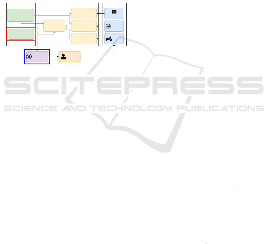
The complete system architecture is illustrated in

Figure (9), where the multibody model and visual-

ization components are highlighted in red and blue,

respectively. The ROS (Robot Operating System)

serves as the communication middleware within this

architecture, facilitating data exchange between dif-

ferent software components, as indicated by the blue

arrows in Figure (9).

Data processing Data interface Motion System

Camera

Sensors

Tractor

Operator

NVIDIA drive PC

Image conversion

Industrial PCs

Sensor signals

conversion

Industrial PCs

Transformation

frame calculation

Linux PC

Data converter

Unreal

Rendering

Matlab PC

Multibody CAD

cosimulation

Linux PC

Pose estimation

(arm & implement)

Figure 9: Real-time implementation architecture.

However, since communication between Sim-

scape and ROS, as well as Unreal Engine and ROS,

requires additional toolboxes or third-party plugins,

the implementation instead utilizes UDP, indicated by

the red arrows. UDP is preferred over TCP because

it can tolerate occasional data loss, as it is solely in-

tended for visualization purposes, where minimizing

delays is critical for providing real-time feedback to

the operator. Data centralization and conversion be-

tween ROS and UDP are managed by the ”Data Con-

verter” component.

3 EXPERIMENTS AND

ASSUMPTIONS

As the setup, models and methods have been de-

scribed in the previous section, this section focuses

on the experiments executed as well as the assump-

tions used. In this research, four main models and

methods need to be validated and are therefore listed

in the following subsections.

3.1 Hydraulic System

The hydraulic model with reduced impact of damp-

ing is validated with the following experiment. The

tractor is placed at standstill, a known payload M

475kg is placed in the implement (i.e a bucket full of

sandbags) and the front-loader is dynamically actu-

ated with different positions while all the signals from

sensors listed in the Section 2.1.3 are logged.

With a ﬁrst simulation, the arm and implement joint

torque can be extracted from a model without virtual

payload and without component density but by using

the hydraulic force measurement as input (see Section

2.2.1). Then a second simulation can be run using the

similar joint states, a virtual known mass in the imple-

ment and component density. Therefore, in the sec-

ond simulation, the ideal joint torque without damp-

ing and stiffness can be directly extracted for a given

payload (and without using the hydraulic force input

from the physical setup). In that way, the hydraulic

model of the ﬁrst simulation can be adapted with a

damping force in order to match the ideal model of

the second simulation.

3.2 Payload Estimation

First, a calibration measurement needs to be per-

formed on the physical setup without payload and

by applying a dynamic movement to the front-loader.

Then a ﬁrst model without virtual payload, with-

out components density but using the hydraulic force

measurement as input is simulated. From the joints

torque computation of that model, the gravitational

parameters of the payload estimation method can be

extracted using the Least Squares Estimation method

as explained in Section 2.3.1. The validation of the

payload estimation method can then use a similar

measurement as for the validation of the hydraulic

system. The pressure and joints state measurement

from the physical setup with a known payload M

475kg are used as inputs for the payload estimation

method that outputs an estimated value of the pay-

load overtime

M. The mean of the estimation error in

percent can be expressed as following:

E = 100 · mean

tε[T

end

]



M − M



(16)

In order to reduce the error caused by unmodeled

dynamic effects, a moving Root Mean Square (RMS)

value of the payload estimation can be computed such

that an operator of the tractor can have a steady esti-

mation of the payload in real-time. The moving RMS

value is computed as follow during the simulation:

MvRMS

mean

tεT

Window

(

) (17)

With T

Window

= 10s the time of the moving win-

dow.

Real-Time Digital Twin for Construction Vehicle Stability Assessment and Visualization with Improved Front-Loader Payload Estimation

273

Finally the overall error of the moving window value

can be expressed in an error in percent as for

MvRMS

= 100 · mean

tε[T

end

]

MvRMS

− M

| (18)

3.3 Stability Assessment and

Visualization

To assess the tractor stability, the stability baseline

and COG position need to be evaluated. Regarding

the stability baseline, this one can be easily extracted

from the physical setup or simulation knowing the

wheels position and the tractor roll and pitch. There-

fore, an accurate estimation of the roll and pitch from

IMU measurement leads to an accurate estimation of

the stability baseline. Although, regarding the COG

position, this one is more difﬁcult to measure on the

physical setup as it requires to know the weight dis-

tribution on the wheels in different vehicle roll-pitch

positions. It was therefore not possible to validate the

COG position with physical measurement. Neverthe-

less, the COG position is ﬁrst impacted by the over-

all components CAD ﬁles accuracy, densities and the

accuracy of their respecting COG position computa-

tion, which is not part of this research. Secondly, the

overall COG is impacted by the front-loader position

and the payload in its implement. The accuracy of the

overall COG position is therefore assumed to be di-

rectly linked to the accuracy of the payload estimation

discussed in the Section 4.2. For the purposes of visu-

alization, it was assumed that the COG moves only in

the forward and upward directions, while remaining

centrally positioned along the vehicle’s width. Conse-

quently, the stability assessment is focused solely on

potential tip-over in the pitch direction. As a result, a

side view is deemed sufﬁcient for operator visualiza-

tion, and a front view—highlighting any asymmetry

across the vehicle’s width—is not necessary.

4 RESULTS AND DISCUSSIONS

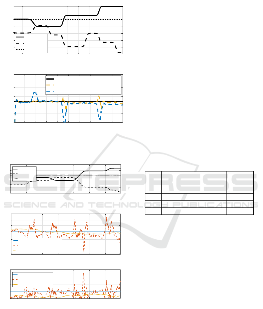
4.1 Hydraulic System

The results of the ﬁrst experiment, described in Sec-

tion 3.1, are shown in the following ﬁgure:

The ﬁrst graph shows the movement of the arm

and the implement in function of the time. The graph

bellow shows the computation of the arm revolute

joint torque for three different models: the torque with

damping directly computed from the setup pressure

measurements in blue, the ideal torque without damp-

ing computed from simulation with a virtual mass

0 10 20 30 40 50 60

Time [s]

-50

Position [deg]

Position of the joints

Arm

Implement

0 10 20 30 40 50 60

Time [s]

Torque [Nm]

Main Arm Revolute Joint

From Setup : with damping model

From Simulation

From Setup

Figure 10: Calibration of Hydraulic Cylinder damping force

model.

in orange and the new torque with reduced damp-

ing from the damping model also computed with the

setup measurements in yellow. It can be observed that

the curve with the damping model is not yet perfectly

matching the ideal torque from simulation but is al-

ready closer than the initial model without damping

force when the front-loader is moving. It is due to

the fact that the complexity of the physical model, in-

cluding several joints damping and friction, is simpli-

ﬁed as one damping force on the hydraulic cylinder

joint. Section 4.2 will show the improvement made

on the payload estimation in dynamic condition using

the damping reduction approach. The new optimized

hydraulic damping parameters are listed in Table 1.

4.2 Payload Estimation

The improvement made in the hydraulic force com-

putation of the previous section is now linked to the

improvement on the payload estimation in the follow-

ing graph:

The ﬁrst graph is again showing the arm and im-

plement position as well as the tractor pitch. In that

experiment the tractor was placed on a ﬂat area with-

out pitch. In the second graph the estimated payload

M from the initial model (in blue) and the model with

reduced impact of the damping (in yellow) are com-

pared to the actual value M

(in black). Both mod-

els are giving a good accuracy when the joints are at

steady state. However, when the front-loader is dy-

namically excited, the method with damping model

is giving a more stable estimation because of the re-

duced impact of the damping that is unmodeled in

the payload estimation method. In that experiment,

the mean of the estimation error in percent

E is re-

duced from 16.1% to 5.9% and

MvRMS

from 12.8%

to 2.9%.

VEHITS 2025 - 11th International Conference on Vehicle Technology and Intelligent Transport Systems

274

5 10 15 20 25 30 35 40 45

Time [s]

-50

-40

-30

-20

-10

Joint position [deg]

Position of the joints

Arm

Implement

Pitch

0 5 10 15 20 25 30 35 40 45

Time [s]

200

400

600

800

1000

Mass [kg]

Payload estimation

Actual

Estimated with damping model

Estimated

Figure 11: Payload estimation: comparison with the damp-

ing model.

15 20 25 30 35 40 45

Time [s]

-60

-40

-20

Joint position [deg]

Position of the joints

Arm

Implement

Pitch

15 20 25 30 35 40 45

Time [s]

380

400

420

440

460

480

500

520

540

Mass [kg]

Payload mass, Mean of Error = 3.88 %

Mean of RMS Window Error = 1.70 %

Actual

Estimated

Estimated RMS Windows

15 20 25 30 35 40 45

Time [s]

Error [%]

Payload mass Estimation error

5% limit

Error

Error RMS Windows

Figure 12: Payload estimation overtime.

The payload estimation of the model with reduced

damping can be analysed in more details with an

other set of data. Here, in the Figure (12), the es-

timated payload

M and the estimated moving RMS

value

MvRMS

are compared to the actual mass M

The third graph displays the absolute error in percent

of those two estimated quantities and a threshold of

5%. The estimated value is again giving a good accu-

racy with an error smaller than 5% with the joints at

steady-state. However, when the front-loader is mov-

ing, a higher error is still remaining because the im-

proved model has not fully removed the impact of the

damping as underlined in Section 4.1. However, it is

shown here that using the moving window RMS value

can drastically reduce the impact of those unmodeled

dynamics. The window RMS error value stays below

5% over the full experiment and has an average value

of 1.7% versus 3.9% for the absolute value. If the

payload in the implement of the construction vehicle

is not expected to dynamically change over time once

the vehicle is loaded, taking an average or a moving

window RMS value is a good solution to deal with

more complex unmodelled dynamic effects. Other-

wise, the method with reduced damping shows an ad-

vantage for the case when the payload is constantly

changing and moving. For example, an excavator that

is digging a hole. The operator should not necessar-

ily immobilize the front loader in order to check the

payload value, therefore improving the productivity.

Table 2: Payload estimation results for multiple values.

MvRMS

[kg] [kg] [%] [kg] [%]

0 2 ∞ 17 ∞

100 115 19.56 109 15.49

200 207 6.96 206 4.40

475 467 3.88 471 1.70

Finally, the overall approach is validated with

multiple payload values. The Table (2) shows the

mean of the estimated mass

M and moving RMS mass

MvRMS

with the corresponding errors. While taking

a moving RMS value is still improving the estimation,

the accuracy decrease with the payload value. The er-

ror in percent is increasing for small payload, how-

ever the absolute error stay bellow 15kg A smaller

payload estimation is more sensitive to the unmod-

elled dynamic effects but also to the accuracy of the

pressure measurements, already including the mass of

the front loader relatively high with respect to a small

payload. However, small payload are less likely to

lead to a vehicle instability while the estimation for

high payload, between 500kg and 1500kg for a trac-

tor front-loader, is expected to be acceptable.

Real-Time Digital Twin for Construction Vehicle Stability Assessment and Visualization with Improved Front-Loader Payload Estimation

275

4.3 Stability Assessment and

Visualization

As introduced in the Section 3.3, the stability of a con-

struction vehicle can be correctly assessed with an ac-

curate estimation of the stability baseline, the COG

position and the suspension system. Regarding the

stability baseline, this one can be evaluated using an

IMU measurement. Secondly, the COG position ac-

curacy is here linked to the accuracy of the payload

estimation presented in Section 4.2.

Figure 13: Visualization towards the operator.

Figure (13) presents the visualization provided to

the operator. It displays the vehicle’s center of grav-

ity (COG), which shifts when the payload changes or

when the tractor adjusts its implement. The yellow-

shaded area represents the stability zone, deﬁned as

the projection of the stability baseline (as discussed

in Section 4.3) along the direction of gravity. When

the COG approaches the boundary of this area, it turns

red, signaling an unstable condition and a heightened

risk of tipping. In addition, the visualization includes

numerical metrics, most notably the estimated pay-

load and the remaining allowable weight before insta-

bility is reached.

5 CONCLUSION

This paper presents the overall story of improvement

of construction vehicle stability assessment and visu-

alization by coupling a front-loader payload estima-

tion method with real-time multibody modeling. The

main goal was to show that the accuracy of multi-

body modelling, for example with MATLAB Sim-

scape Multibody software, can be used to improve a

payload estimation method based on simpliﬁed mo-

tion equations. This paper underlines those improve-

ments by reducing the impact of joints damping on the

payload estimation and by allowing to run in parallel

and in real-time a multibody model including suspen-

sions system and Center Of Gravity computation.

Regarding the payload estimation, the multibody

model is used to reduce the impact of joint damp-

ing by comparing joints torque from a physical setup

and the ideal joint torque without damping in simu-

lation. It therefore allows to quantify the impact of

damping and remove it from the physical setup joint

torque used for the payload estimation. The mean of

the estimation moving window RMS error can be re-

duced from 12.8% to 2.9%. For real-time integration

on a working vehicle, using such a solution with re-

duced impact of damping is better than just taking a

mean on a moving windows value for vehicles that

are constantly in movement or constantly changing

the payload (e.g. a excavator digging an hole or mov-

ing sand).

The payload estimation and stability assessment

have been integrated in a real-time system with a 3D

visualization that is designed to provide the vehicle

operator with intuitive feedback on stability, focus-

ing on tip-over risks in the pitch direction. Commu-

nication between system components was achieved

primarily through ROS and UDP. The system effec-

tively visualizes the vehicle’s center of gravity, stabil-

ity zone, and key metrics, allowing operators to mon-

itor and maintain safe operational conditions.

5.1 Outlook

The aims of this paper is to introduce a way to couple

accurate multibody modelling with a more simpliﬁed

payload estimation method using motion equations

and integrate it in a real-time system with a 3D visual-

ization. While some examples are demonstrated and

validated within this research, several other investiga-

tions and modelling improvement could be further ex-

plored. First, the modelling of a moving vehicle could

be developed. It allows to validate the impact of sus-

pension on the stability behaviour but could also be

used to improve the payload estimation method by re-

ducing the impact of vehicle roll and pitch in case no

IMU’s measurements are available. Moreover, adding

weight distribution measurement on the wheels of the

physical setup could allow a more accurate validation

of the center of gravity position and overall stability

assessment. Finally, the payload estimation method

could be further improved by modelling and reduc-

ing the impact of other unmodelled effects in the sim-

pliﬁed motion equations such as joint frictions, hy-

draulics delay, components ﬂexibility, etc.

VEHITS 2025 - 11th International Conference on Vehicle Technology and Intelligent Transport Systems

276

ACKNOWLEDGEMENTS

This research is part of the CADAIVision SBO

project funded and supported by Flanders Make vzw,

the strategic research center for the manufacturing in-

dustry.

REFERENCES

AlliedMarketResearch (2024). Construction vehicles mar-

ket size, share, competitive landscape and trend anal-

ysis report, by solution, by equipment, by type, by ap-

plication and, by industry : Global opportunity anal-

ysis and industry forecast, 2023-2032. Construction

Vehicles Market.

Baker, V. and Guzzomi, A. L. (2013). A model and com-

parison of 4-wheel-drive ﬁxed-chassis tractor rollover

during phase i. Biosystems Engineering, 116(2):179–

189.

Bennett, N., Walawalkar, A., and Schindler, C. (2014). Pay-

load estimation in excavators: Model-based evalua-

tion of current payload estimation systems.

Cordos¸, N. and TodoruT¸ , A. (2019). Inﬂuences of the sus-

pensions characteristics on the vehicle stability. In

Burnete, N. and Varga, B. O., editors, Proceedings

of the 4th International Congress of Automotive and

Transport Engineering (AMMA 2018), pages 808–

813, Cham. Springer International Publishing.

Cuong, D., Zhu, S., Hung, D., and Ngoc, N. (2013). Study

on the vertical stiffness and damping coefﬁcient of

tractor tire using semi-empirical model. Hue Univer-

sity Journal of Science, 83:5–15.

Edwards, D., Parn, E. A., Sing, M. C., and Thwala, W. D.

(2019). Risk of excavators overturning: Determining

horizontal centrifugal force when slewing freely sus-

pended loads. Engineering, construction, and archi-

tectural management, 26(3):479–498.

Ferlibas, M. and Ghabcheloo, R. (2021). The 17th scandi-

navian international conference on ﬂuid power. Hue

University Journal of Science.

Gralak, M. and Walu

s, K. (2024). A model of an extending

front loader. Applied Sciences, 14:3948.

Huo, D., Chen, J., Zhang, H., Shi, Y., and Wang, T. (2023).

Intelligent prediction for digging load of hydraulic ex-

cavators based on rbf neural network. Measurement,

206:112210.

Ishihara, S., Kanazawa, A., and Narikawa, R. (2021). Re-

alization of excavator loading operation by nonlinear

model predictive control with bucket load estimation.

In IFAC-PapersOnLine, volume 54, pages 20–25. El-

sevier Ltd.

Lysych, M. N. (2020). Study driving dynamics of the

machine-tractor unit on a virtual stand with ob-

stacles. Journal of Physics: Conference Series,

1515(4):42079–.

MarkwideResearch (2024). Construction vehicles mar-

ket analysis- industry size, share, research report, in-

sights, covid-19 impact, statistics, trends, growth and

forecost 2024-2032. Automotive and Transportation,

pages 1–263.

Mitrev, R. and Marinkovi

c, D. (2019). Numerical study

of the hydraulic excavator overturning stability during

performing lifting operations. Advances in mechani-

cal engineering, 11(5):168781401984177–133.

Murphy, D. (2022). Tractor Stability and Instability. https:

//extension.psu.edu/tractor-stability-and-instability.

Updated : July 15, 2022.

New Holland Agriculture (2024). Front Axle and

Suspension. https://agriculture.newholland.com/

apac/th-th/equipment/products/agricultural-tractors/

t7-heavy-duty/detail/front-axle-and-suspension.

Accessed: 2024-08-06.

Pavlov, N. and Dacova, D. (2021). A multibody model of

a wheel loader with pneumatic boom suspension and

proving ground testing. IOP Conference Series: Ma-

terials Science and Engineering, 1031:012009.

Robyns, S., Heerwegh, W., and Weckx, S. (2024). A dig-

ital twin of an off highway vehicle based on a low

cost camera. Procedia Computer Science, 232:2366–

2375. 5th International Conference on Industry 4.0

and Smart Manufacturing (ISM 2023).

Tafazoli, S., Lawrence, P. D., and Salcudean, S. E.

(1999). Identiﬁcation of inertial and friction parame-

ters for excavator arms. IEEE Trans. Robotics Autom.,

15:966–971.

Zhu, Q., Yang, C., Hu, H., and Wu, X. (2021). Building a

novel dynamics rollover model for critical instability

state analysis of articulated multibody vehicles. Inter-

national Journal of Heavy Vehicle Systems, 28:329–

352.

Real-Time Digital Twin for Construction Vehicle Stability Assessment and Visualization with Improved Front-Loader Payload Estimation

277