Optimizing Sensor Redundancy in Sequential Decision-Making Problems

Jonas N

ußlein, Maximilian Zorn, Fabian Ritz, Jonas Stein, Gerhard Stenzel, Julian Sch

onberger,

Thomas Gabor and Claudia Linnhoff-Popien

Institute of Computer Science, LMU Munich, Germany

ﬁ

Keywords:

Reinforcement Learning, Sensor Redundancy, Robustness, Optimization.

Abstract:

Reinforcement Learning (RL) policies are designed to predict actions based on current observations to max-

imize cumulative future rewards. In real-world, i.e. not simulated, environments, sensors are essential for

measuring the current state and providing the observations on which RL policies rely to make decisions. A

signiﬁcant challenge in deploying RL policies in real-world scenarios is handling sensor dropouts, which can

result from hardware malfunctions, physical damage, or environmental factors like dust on a camera lens. A

common strategy to mitigate this issue is to use backup sensors, though this comes with added costs. This

paper explores the optimization of backup sensor conﬁgurations to maximize expected returns while keeping

costs below a speciﬁed threshold, C. Our approach uses a second-order approximation of expected returns

and includes penalties for exceeding cost constraints. The approach is evaluated across eight OpenAI Gym

environments and a custom Unity-based robotic environment (RobotArmGrasping). Empirical results demon-

strate that our quadratic program effectively approximates real expected returns, facilitating the identiﬁcation

of optimal sensor conﬁgurations.

1 INTRODUCTION

Reinforcement Learning (RL) has emerged as a

prominent technique for solving sequential decision-

making problems, paving the way for highly au-

tonomous systems across diverse ﬁelds. From

controlling complex physical systems like tokamak

plasma (Degrave et al., 2022) to mastering strategic

games such as Go (Silver et al., 2018), RL has demon-

strated its potential to revolutionize various domains.

However, when transitioning from controlled envi-

ronments to real-world applications, RL faces sub-

stantial challenges, particularly in dealing with sen-

sor dropouts. In critical scenarios, such as healthcare

or autonomous driving, the failure of sensors can re-

sult in suboptimal decisions or even catastrophic out-

comes.

The core of RL decision-making lies in its reliance

on continuous, accurate observations of the environ-

ment, often captured through sensors. When these

sensors fail to provide reliable data — whether due to

hardware malfunctions, environmental interference,

or physical damage — the performance of RL policies

can degrade signiﬁcantly (Dulac-Arnold et al., 2019).

In domains such as aerospace, healthcare, nuclear en-

ergy, and autonomous vehicles, the consequences of

sensor failures are particularly severe. This vulner-

ability highlights the importance of addressing sen-

sor dropout to ensure the robustness of RL systems

in real-world applications. Thus, improving the re-

silience of RL systems to sensor dropouts is not just

desirable—it is critical for ensuring their safe and re-

liable deployment in mission-critical applications.

One common approach to mitigate the risks of

sensor dropouts is the implementation of redundant

backup sensors. These backup systems provide an ad-

ditional layer of security, stepping in when primary

sensors fail, thereby maintaining the availability of

crucial data. While redundancy can enhance system

resilience, it also introduces signiﬁcant costs, and not

all sensor dropouts result in performance degrada-

tion severe enough to justify the investment in back-

ups. This paper presents a novel approach to op-

timizing backup sensor conﬁgurations in RL-based

systems. Our method focuses on balancing system

performance — quantiﬁed by expected returns in a

Markov Decision Process (MDP) — and the costs as-

sociated with redundant sensors.

This publication was created as part of the Q-Grid

project (13N16179) under the “quantum technologies –

from basic research to market” funding program, supported

by the German Federal Ministry of Education and Research.

Nüßlein, J., Zorn, M., Ritz, F., Stein, J., Stenzel, G., Schönberger, J., Gabor, T. and Linnhoff-Popien, C.

Optimizing Sensor Redundancy in Sequential Decision-Making Problems.

DOI: 10.5220/0013086700003890

Paper published under CC license (CC BY-NC-ND 4.0)

In Proceedings of the 17th International Conference on Agents and Artiﬁcial Intelligence (ICAART 2025) - Volume 1, pages 245-252

ISBN: 978-989-758-737-5; ISSN: 2184-433X

245

2 BACKGROUND

2.1 Markov Decision Processes (MDP)

Sequential Decision-Making problems are frequently

modeled as Markov Decision Processes (MDPs). An

MDP is deﬁned by the tuple E = ⟨S, A,T, r, p

,γ⟩,

where S represents the set of states, A is the set of

actions, and T (s

t+1

| s

) is the probability density

function (pdf) that governs the transition to the next

state s

t+1

after taking action a

in state s

. The pro-

cess is considered Markovian because the transition

probability depends only on the current state s

and

the action a

, and not on any prior states s

τ<t

The function r : S ×A → R assigns a scalar reward

to each state-action pair (s

). The initial state is

sampled from the start-state distribution p

, and γ ∈

[0,1) is the discount factor, which applies diminishing

weight to future rewards, giving higher importance to

immediate rewards.

A deterministic policy π : S → A is a mapping

that assigns an action to each state. The return R =

∑

∞

t=0

· r(s

) is the total (discounted) sum of re-

wards accumulated over an episode. The objective,

typically addressed by Reinforcement Learning (RL),

is to ﬁnd an optimal policy π

∗

that maximizes the ex-

pected cumulative return:

∗

= argmax

∞

∑

t=0

· r(s

) | π

Actions a

are selected according to the policy π.

In Deep Reinforcement Learning (DRL), where state

and action spaces can be large and continuous, the

policy π is often represented by a neural network

(s)

with parameters φ, which are learned through training

(Sutton and Barto, 2018).

2.2 Quadratic Unconstrained Binary

Optimization (QUBO)

Quadratic Unconstrained Binary Optimization

(QUBO) is a combinatorial optimization problem

deﬁned by a symmetric, real-valued (m × m) matrix

Q, and a binary vector x ∈ B

. The objective of

a QUBO problem is to minimize the following

quadratic function:

∗

= argmin

H(x) = argmin

∑

i=1

∑

j=i

i j

(1)

The function H(x) is commonly referred to as the

Hamiltonian, and in this paper, we refer to the matrix

Q as the “QUBO matrix”.

The goal is to ﬁnd the optimal binary vector x

∗

that minimizes the Hamiltonian. This task is known

to be NP-hard, making it computationally intractable

for large instances without specialized techniques.

QUBO is a signiﬁcant problem class in combinato-

rial optimization, as it can represent a wide range of

problems. Moreover, several specialized algorithms

and hardware platforms, such as quantum annealers

and classical heuristics, have been designed to solve

QUBO problems efﬁciently (Morita and Nishimori,

2008; Farhi and Harrow, 2016; N

ußlein et al., 2023b;

ußlein et al., 2023a).

Many well-known combinatorial optimization

problems, such as Boolean satisﬁability (SAT), the

knapsack problem, graph coloring, the traveling

salesman problem (TSP), and the maximum clique

problem, have been successfully reformulated as

QUBO problems (Choi, 2011; Lodewijks, 2020;

Choi, 2010; Glover et al., 2019; Lucas, 2014). This

versatility makes QUBO a powerful tool for solving a

wide variety of optimization tasks, including the one

addressed in this paper.

3 ALGORITHM

3.1 Problem Deﬁnition

Let π be a trained agent operating within an MDP E.

At each timestep, the agent receives an observation

o ∈ R

, which is collected using n sensors {s

}

1≤i≤n

Each sensor s

produces a vector o

, and the full ob-

servation o is formed by concatenating these vectors:

o = [o

,.. . ,o

]. The complete observation o has

dimension |o| =

∑

At the start of an episode, each sensor s

may drop

out with probability d

∈ [0,1], meaning it fails to pro-

vide any meaningful data for the entire episode. In the

event of a dropout, the sensor’s output is set to o

= 0

for the rest of the episode.

If π is represented as a neural network, it is evident

that the performance of π, quantiﬁed as the expected

return, will degrade as more sensors drop out. To mit-

igate this, we can add backup sensors. However, in-

corporating a backup sensor s

incurs a cost c

∈ N,

representing the expense associated with adding that

redundancy.

The task is to ﬁnd the optimal backup sensor con-

ﬁguration that maximizes the expected return while

keeping the total cost of the backups within a prede-

ﬁned budget C ∈ N. Let x ∈ B

be a vector of binary

decision variables, where x

= 1 indicates the inclu-

sion of a backup for sensor s

. If E

d,π,x

[R] represents

the expected return while using backup conﬁguration

ICAART 2025 - 17th International Conference on Agents and Artiﬁcial Intelligence

246

x, the optimization problem can be formulated with

both a soft and hard constraint:

∗

= argmax

d,π,x

[R] s.t.

∑

i=1

≤ C (2)

An illustration of this problem is provided in Fig-

ure 1. In the next section, we describe a method to

transform this problem into a QUBO representation.

3.2 SensorOpt

There are potentially 2

possible combinations of sen-

sor dropout conﬁgurations, making it computationally

expensive to evaluate all of them directly. Since we

only have a limited number of episodes B ∈ N to sam-

ple from the environment E, we opted for a second-

order approximation of E

d,π,x

[R] to reduce the com-

putational burden while still capturing meaningful in-

teractions between sensor dropouts.

To compute this approximation, we ﬁrst calculate

the probability q(d) that at most two sensors drop out

in an episode:

q(d) =

∏

i=1

(1 − d

) +

∑

i=1

∏

j̸=i

(1 − d

)

∑

i=1

∑

j<i

∏

l̸=i, j

(1 − d

)

Next, we estimate the expected return

(i, j)

for

each pair of sensors (s

) dropping out. This can

be efﬁciently achieved using Algorithm 1, which

samples the episode return E

(i, j)

(π) using policy π

with sensors s

and s

removed. The algorithm be-

gins by calculating two return values for each sen-

sor pair. It then iteratively selects the sensor pair

with the highest momentum of the mean return, de-

ﬁned as |R

(i, j)

[: −1] − R

(i, j)

|. Here, R

(i, j)

[: −1] de-

notes the mean of all previously sampled returns for

the sensor pair (s

), excluding the most recent re-

turn, while R

(i, j)

represents the mean including the

most recent return. The difference between these two

values measures the momentum, capturing how much

the expected return is changing as more episodes are

sampled.

We base the selection of sensor pairs on mo-

mentum rather than return variance to differen-

tiate between aleatoric and epistemic uncertainty

(Valdenegro-Toro and Mori, 2022). Momentum is

less sensitive to aleatoric uncertainty, making it a

more reliable indicator in this context.

A simpler, baseline approach to estimate

(i, j)

would be to divide the budget B of episodes evenly

across all sensor pairs (s

). In this Round Robin ap-

proach, we sample k =

n(n+1)/2

episodes for each sen-

sor pair and estimate

(i, j)

as the empirical mean. In

the Experiments section, we compare our momentum-

based approach from Algorithm 1 against this naive

Round Robin method to highlight its efﬁciency and

accuracy.

Once we have estimated all the values of

(i, j)

we can compute the overall expected return

R(d) for

a given dropout probability vector d, again using a

second-order approximation:

R(d) =

q(d)

∏

i=1

(1 − d

) +

∑

i=1

(i,i)

∏

j̸=i

(1 − d

)

∑

i=1

∑

j<i

(i, j)

∏

l̸=i, j

(1 − d

)

Now we can calculate the advantage of using a backup

for sensor s

vs. using no backup sensor for s

∆

(i,i)

(d) =

R(d

{i}

) −

R(d)

with

(

if i ∈ A,

if i /∈ A.

When a backup sensor is used for sensor s

, the new

dropout probability for s

becomes d

← d

, since

the system will only fail to provide an observation if

both the primary and backup sensors drop out. We

adopt the notation d

to represent the updated dropout

probabilities when backup sensors from set A are in

use. For example, if the dropout probability vector is

d = (0.2,0.5,0.1) and a backup is used for sensor 1,

the updated vector becomes d

= (0.2,0.25, 0.1), as

the backup reduces the dropout probability for sensor

1 while sensors 0 and 2 remain unchanged.

We can now compute the joint advantage of using

backups for both sensors s

and s

. This joint advan-

tage is not simply the sum of the individual advan-

tages of using backups for each sensor in isolation:

∆

(i, j)

(d) =

R(d

{i, j}

)−

R(d) −∆

(i,i)

(d) −∆

( j, j)

(d)

This formula accounts for the interaction between

the two sensors, reﬂecting the fact that their joint con-

tribution to the expected return is inﬂuenced by how

the presence of both backup sensors affects the system

as a whole, beyond just the sum of their individual

contributions. This interaction term is crucial when

optimizing backup sensor conﬁgurations, as it helps

Optimizing Sensor Redundancy in Sequential Decision-Making Problems

247

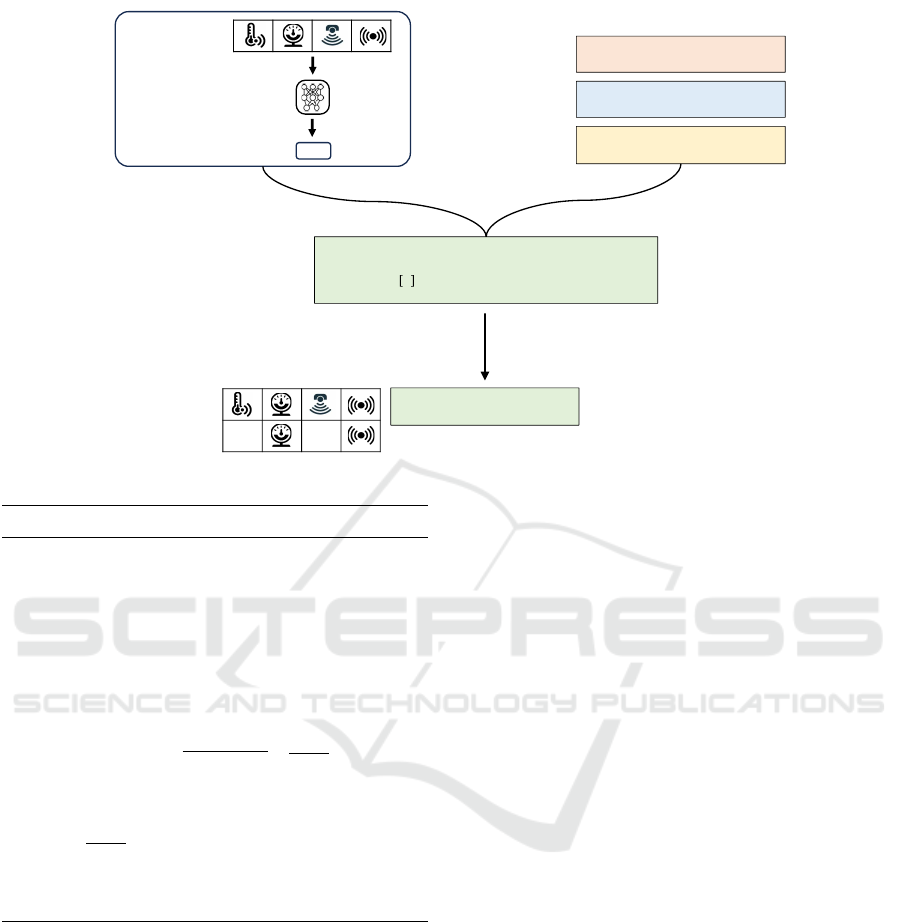
Objective:









 s.t.













  (maximally allowed costs)

Costs for adding a backup sensor:

     

Probability for each sensor to drop out:

     

Binary decision variables for using

backup sensors:   



solve this NP-hard problem using

any QUBO solver

optimal set of backup sensors:





    

observation

  



(here via

   sensors)

action   



policy 

trained 

  



Figure 1: An illustration of our approach for optimizing the backup sensor conﬁguration.

Algorithm 1: Estimating

(i, j)

Input: budget of episodes to run B ∈ N

# sensors n ∈ N

MDP E

trained policy π

(i, j)

= [E

(i, j)

(π),E

(i, j)

(π)] ∀i < j,(i, j) ∈ [1,n]

for e = 1 to B − n(n + 1) do

(i, j) = arg max

(i, j)

| R

(i, j)

[: −1] − R

(i, j)

.append



(i, j)

(π)



end for

(i, j)

= R

(i, j)

// expected return = mean

empirical return

return all

(i, j)

capture the diminishing or synergistic returns that can

occur when multiple sensors are backed up together.

With these components in hand, we can now for-

mulate the QUBO problem for the sensor optimiza-

tion task deﬁned in (2). The soft constraint H

so f t

cap-

tures the optimization of the expected return, approxi-

mated by the change in return ∆

(i,i)

(d) for individual

sensors and ∆

(i, j)

(d) for sensor pairs:

so f t

∑

i=1

· ∆

(i,i)

(d) +

∑

i< j

· ∆

(i, j)

(d)

Here, x

are binary decision variables where x

= 1

indicates that a backup sensor is added for sensor s

This formulation ensures that the algorithm optimizes

the expected return based on the speciﬁc backup con-

ﬁguration.

To enforce the cost constraint, we introduce a

hard constraint H

hard

, which penalizes conﬁgurations

where the total cost exceeds the speciﬁed budget C:

hard

∑

i=1

n+1+⌈log

(C)⌉

∑

i=n+1

(i−n−1)

−C

The expression

∑

i=1

represents the total cost

of the selected backup sensors, and the second term

accounts for the binary encoding of the cost con-

straint, ensuring that no conﬁguration exceeds the

budget C.

Finally, we introduce a scaling factor α to balance

the contributions of the soft and hard constraints:

α =

∑

i=1

|∆

(i,i)

(d)| +

∑

i< j

|∆

(i, j)

(d)|

The overall QUBO objective function is then

given by:

H = −H

so f t

+ β · α · H

hard

(3)

Here, H

so f t

approximates the expected return

d,π,x

[R], while H

hard

ensures that the total cost re-

mains within the allowable budget. The parameter

β is a hyperparameter that controls the trade-off be-

tween maximizing the expected return and enforcing

the cost constraint.

Algorithm SensorOpt summarizes our approach

for optimizing sensor redundancy conﬁgurations.

ICAART 2025 - 17th International Conference on Agents and Artiﬁcial Intelligence

248

This algorithm uses the QUBO formulation to ﬁnd the

optimal backup sensor conﬁguration, balancing per-

formance improvements with budget constraints.

Algorithm 2: - SensorOpt: Calculating best sensor backup

conﬁguration.

Input: # sensors n ∈ N

dropout probability for each sensor d ∈

[0,1]

costs for each backup sensor c ∈ N

maximally allowed costs C ∈ N

budget of episodes to run B ∈ N

MDP E

trained policy π

← E(π) // expected return with no sensor

dropouts

(i, j)

← use Algorithm 1 (B,n,E,π)

Q ← create QUBO-matrix using formula (3)

∗

= argmin

Qx // solve using any QUBO

solver,

e.g. Tabu Search

// x ∈ B

, m = n + ⌈log

(C)⌉

return x

∗

[: n] // ﬁrst n bits of x

∗

encode the

optimal

sensor backup conﬁguration

For a given problem instance (n,d,c,C,B, E,π),

α is a constant while β ∈ [0,1] is a hyperparameter

we need to choose by hand. The number of boolean

decision variables our approach needs is determined

by m = n + ⌈log

(C)⌉.

Proposition 1. The optimization problem described

in (2) belongs to complexity class NP-hard.

Proof. We can prove that the problem described in

(2) belongs to NP-hard by reducing another prob-

lem W , that is already known to be NP-hard, to

it. Since this would imply that, if we have a

polynomial algorithm for solving (2), we could

solve any problem instance w ∈ W using this algo-

rithm. We choose W to be Knapsack (Salkin and

De Kluyver, 1975) which is known to be NP-hard.

For a given Knapsack instance (n

(1)

)

consisting of n

(1)

items with values v

(1)

, costs c

(1)

and maximal costs C

(1)

we can reduce this to a

problem instance (n

(2)

,E) from (2)

via: n

(2)

= n

(1)

, d

(2)

= 0, c

(2)

= c

(1)

, C

(2)

= C

(1)

For each possible x we deﬁne an individual MDP

: S = {s

terminal

},A = {a

},T (s

terminal

) =

1,r(s

) = x · v, p

) = 1, γ = 1. The expected

return E

d,π,x

[R] will therefore be E

d,π,x

[R] = x · v.

4 RELATED WORK

Robust Reinforcement Learning (Moos et al., 2022;

Pinto et al., 2017) is a sub-discipline within RL that

tries to learn robust policies in the face of several

types of perturbations in the Markov Decision Process

which are (1) Transition Robustness due to a proba-

bilistic transition model T (s

t+1

) (2) Action Ro-

bustness due to errors when executing the actions (3)

Observation Robustness due to faulty sensor data.

There is a bulk of papers dealing with Observation

Robustness (L

utjens et al., 2020; Mandlekar et al.,

2017; Pattanaik et al., 2017). However, the vast ma-

jority is about handling noisy observations, meaning

that the true state lies within an ε-ball of the perceived

observation. In these scenarios, an adversarial an-

tagonist is usually used in the training process that

adds noise to the observation, trying to decrease the

expected return, while the agent tries to maximize it

(Liang et al., 2022; L

utjens et al., 2020; Mandlekar

et al., 2017; Pattanaik et al., 2017). In our problem

setting, however, the sensors are not noisy in the sense

of ε-disturbance, but they can drop out entirely.

Another line of research is about the framework

Action-Contingent Noiselessly Observable Markov

Decision Processes (ACNO-MDP) (Nam et al., 2021;

Koseoglu and Ozcelikkale, 2020). In this framework,

observing (measuring) the current state s

comes with

costs. The agent therefore needs to learn when ob-

serving a state is crucially important for informed ac-

tion decision making and when not. The action space

is extended by two additional actions {observe, not

observe} (Beeler et al., 2021). Not observe, however,

affects all sensors.

Important other related work comes from Safe Re-

inforcement Learning (Gu et al., 2022; Dulac-Arnold

et al., 2019). In (Dulac-Arnold et al., 2019) the prob-

lem of sensors dropping out is already mentioned and

analyzed. However, they only examine the scenario in

which the sensor drops out for z ∈ N timesteps. There-

fore they can use Recurrent Neural Networks for rep-

resenting the policy that mitigates this problem.

Our approach for optimizing the sensor redun-

dancy conﬁguration given a maximal cost C bears

similarity to Knapsack (Salkin and De Kluyver, 1975;

Martello and Toth, 1990). In (Lucas, 2014) a QUBO

formulation for Knapsack was already introduced and

(Quintero and Zuluaga, 2021) provides a study re-

garding the trade-off parameter for the hard- and soft-

constraint. The major difference between the original

Knapsack problem and our problem is that in Knap-

Optimizing Sensor Redundancy in Sequential Decision-Making Problems

249

Figure 2: Proof-of-concept: this plot shows the real expected return and the approximated expected return E

d,π,x

[R] ≈

− x

Q x +

R(d) when using a backup sensor conﬁguration x. The conﬁgurations (x-axis) are sorted according to the real

return.

sack, the value of a collection of items is the sum of

all item values: W =

∑

. In our problem formu-

lation this, however, doesn’t hold. We therefore pro-

posed a second-order approximation for representing

the soft-constraint.

To the best of our knowledge, this paper is the ﬁrst

to address the optimization of sensor redundancy in

sequential decision-making environments.

5 EXPERIMENTS

In this Experiments section we want to evaluate our

algorithm SensorOpt. Speciﬁcally, we want to exam-

ine the following hypotheses:

1. Hamiltonian H of formula (3) approximates the

real expected returns.

2. Our algorithm SensorOpt can ﬁnd optimal sensor

backup conﬁgurations.

3. Algorithm 1 approximates the expected returns

(i, j)

faster than with Round Robin.

5.1 Proof-of-Concept

To test how well our QUBO formulation (a second-

order approximation) approximates the real expected

return for each possible sensor redundancy conﬁgu-

ration x we created a random problem instance and

determined the Real Expected Returns E

d,π,x

[R] and

the Approximated Expected Returns:

d,π,x

[R] ≈ − x

Q x +

R(d)

Note that in general a QUBO-matrix can be lin-

early scaled by a scalar g without altering the order

of the solutions regarding solution quality. Figure

2 shows the two resulting graphs where the x-axis

represents all possible sensor backup conﬁgurations

x and the y-axis the expected return. We have sorted

the conﬁgurations according to their real expected re-

turns. The key ﬁnding in this plot is that the ap-

proximation is quite good even though it is not per-

fect for all x. But the relative performance is still in-

tact, meaning especially that the best solution in our

approximation is also the best solution regarding the

real expected returns. We can therefore verify the ﬁrst

hypothesis that our Hamiltonian H approximates the

real expected returns. But as with any approximation,

it can contain errors.

5.2 RobotArmGrasping Environment

The RobotArmGrasping domain is a robotic simula-

tion based on a digital twin of the Niryo One

which is

available in the Unity Robotics Hub

. It uses Unity’s

built-in physics engine and models a robot arm that

can grasp and lift objects.

5.3 Main Experiments

Next, we tested if SensorOpt can ﬁnd optimal sensor

backup conﬁgurations in well-known MDPs. We used

8 different OpenAI Gym environments (Brockman

et al., 2016). Additionally, we created a more realistic

and industry-relevant environment RobotArmGrasp-

ing based on Unity. In this environment, the goal of

the agent is to pick up a cube and lift it to a desired lo-

cation. The observation space is 20-dimensional and

the continuous action space is 5-dimensional.

https://niryo.com/niryo-one/

https://github.com/Unity-Technologies/

Unity-Robotics-Hub

ICAART 2025 - 17th International Conference on Agents and Artiﬁcial Intelligence

250

Table 1: Results of our algorithm SensorOpt on 9 different environments compared against the true optimum, determined via

brute force and the baselines when using no additional backup sensors and all possible backup sensors. We solved the QUBO

created in SensorOpt using Tabu Search. Note that All Backups is not a valid solution to the problem presented in formula (2),

since the cost of using all backup sensors exceeds the threshold C. Due to the exponential complexity of conducting a brute

force search for the optimal conﬁguration, it was feasible to apply this approach only to the ﬁrst four environments.

ENVIRONMENT SENSOROPT OPTIMUM* NO BACKUPS ALL BACKUPS

CARTPOLE-V1 493.3 493.3 424.0 498.7

ACROBOT-V1 -86.73 -86.73 -91.38 -83.01

LUNARLANDER-V2 241.5 241.5 200.1 249.5

HOPPER-V2 2674 2674 1979 3221

HALFCHEETAH-V2 9643 - 8119 10711

WALKER2D-V2 3388 - 2402 4097

BIPEDALWALKER-V3 215.5 - 160.2 273.0

SWIMMER-V2 329.6 - 272.6 341.7

ROBOTARMGRASPING 29.41 - 22.27 30.41

In all experiments, we sampled each dropout prob-

ability d

, cost c

, and maximum costs C uniformly out

of a ﬁxed set. For simplicity, we restricted the costs c

in our experiments to be integers.

For the 8 OpenAI Gym environments we used

as the trained policies SAC- (for continuous action

spaces) or PPO- (for discrete action spaces) models

from Stable Baselines 3 (Rafﬁn et al., 2021). For our

RobotArmGrasping environment we trained a PPO

agent (Schulman et al., 2017) for 5M steps. We

then solved the sampled problem instances using Sen-

sorOpt. We optimized the QUBO in SensorOpt using

Tabu Search, a classical meta-heuristic. Further, we

calculated the expected returns when using no backup

sensors (No Backups) and all n backup sensors (All

Backups). For the four smallest environments Cart-

Pole, Acrobot, LunarLander and Hopper we also de-

termined the true optimal backup sensor conﬁguration

∗

using brute force. This was however not possible

for larger environments.

For each environment, we sampled 10 problem in-

stances. Note that using all backup sensors is not a

valid solution regarding the problem deﬁnition in for-

mula (2) since the costs would exceed the maximally

allowed costs

∑

> C. All results are reported in

Table 2.

The results show that SensorOpt found the op-

timal sensor redundancy conﬁguration in the ﬁrst

four environments for which we were computation-

ally able to determine the optimum using brute force.

6 CONCLUSION

Sensor dropouts present a major challenge when de-

ploying reinforcement learning (RL) policies in real-

world environments. A common solution to this prob-

lem is the use of backup sensors, though this approach

introduces additional costs. In this paper, we tackled

the problem of optimizing backup sensor conﬁgura-

tions to maximize expected return while ensuring the

total cost of added backup sensors remains below a

speciﬁed threshold, C.

Our method involved using a second-order ap-

proximation of the expected return, E

d,π,x

[R] ≈

−x

Qx +

R(d), for any given backup sensor conﬁg-

uration x ∈ B

. We incorporated a penalty for conﬁg-

urations that exceeded the maximum allowable cost,

C, and optimized the resulting QUBO matrices Q us-

ing the Tabu Search algorithm.

We evaluated our approach across eight OpenAI

Gym environments, as well as a custom Unity-based

robotic scenario, RobotArmGrasping. The results

demonstrated that our quadratic approximation was

sufﬁciently accurate to ensure that the optimal con-

ﬁguration derived from the approximation closely

matched the true optimal sensor conﬁguration in prac-

tice.

REFERENCES

Beeler, C., Li, X., Bellinger, C., Crowley, M., Fraser, M.,

and Tamblyn, I. (2021). Dynamic programming with

incomplete information to overcome navigational un-

certainty in a nautical environment. arXiv preprint

arXiv:2112.14657.

Brockman, G., Cheung, V., Pettersson, L., Schneider, J.,

Schulman, J., Tang, J., and Zaremba, W. (2016). Ope-

nai gym. arXiv preprint arXiv:1606.01540.

Choi, V. (2010). Adiabatic quantum algorithms for the

NP-complete maximum-weight independent set, ex-

act cover and 3SAT problems.

Choi, V. (2011). Different adiabatic quantum optimization

algorithms for the NP-complete exact cover and 3SAT

problems.

Degrave, J., Felici, F., Buchli, J., Neunert, M., Tracey, B.,

Carpanese, F., Ewalds, T., Hafner, R., Abdolmaleki,

A., de Las Casas, D., et al. (2022). Magnetic con-

Optimizing Sensor Redundancy in Sequential Decision-Making Problems

251

trol of tokamak plasmas through deep reinforcement

learning. Nature, 602(7897):414–419.

Dulac-Arnold, G., Mankowitz, D., and Hester, T. (2019).

Challenges of real-world reinforcement learning.

arXiv preprint arXiv:1904.12901.

Farhi, E. and Harrow, A. W. (2016). Quantum supremacy

through the quantum approximate optimization algo-

rithm. arXiv preprint arXiv:1602.07674.

Glover, F., Kochenberger, G., and Du, Y. (2019). Quantum

bridge analytics I: A tutorial on formulating and using

QUBO models.

Gu, S., Yang, L., Du, Y., Chen, G., Walter, F., Wang, J.,

Yang, Y., and Knoll, A. (2022). A review of safe re-

inforcement learning: Methods, theory and applica-

tions. arXiv preprint arXiv:2205.10330.

Koseoglu, M. and Ozcelikkale, A. (2020). How to miss

data? reinforcement learning for environments with

high observation cost. In ICML Workshop on the Art

of Learning with Missing Values (Artemiss).

Liang, Y., Sun, Y., Zheng, R., and Huang, F. (2022). Ef-

ﬁcient adversarial training without attacking: Worst-

case-aware robust reinforcement learning. Advances

in Neural Information Processing Systems, 35:22547–

22561.

Lodewijks, B. (2020). Mapping NP-hard and NP-complete

optimisation problems to quadratic unconstrained bi-

nary optimisation problems.

Lucas, A. (2014). Ising formulations of many NP problems.

utjens, B., Everett, M., and How, J. P. (2020). Certiﬁed ad-

versarial robustness for deep reinforcement learning.

In conference on Robot Learning, pages 1328–1337.

PMLR.

Mandlekar, A., Zhu, Y., Garg, A., Fei-Fei, L., and Savarese,

S. (2017). Adversarially robust policy learning:

Active construction of physically-plausible perturba-

tions. In 2017 IEEE/RSJ International Conference on

Intelligent Robots and Systems (IROS), pages 3932–

3939. IEEE.

Martello, S. and Toth, P. (1990). Knapsack problems: algo-

rithms and computer implementations. John Wiley &

Sons, Inc.

Moos, J., Hansel, K., Abdulsamad, H., Stark, S., Clever, D.,

and Peters, J. (2022). Robust reinforcement learning:

A review of foundations and recent advances. Ma-

chine Learning and Knowledge Extraction, 4(1):276–

315.

Morita, S. and Nishimori, H. (2008). Mathematical founda-

tion of quantum annealing. Journal of Mathematical

Physics, 49(12).

Nam, H. A., Fleming, S., and Brunskill, E. (2021). Re-

inforcement learning with state observation costs in

action-contingent noiselessly observable markov deci-

sion processes. Advances in Neural Information Pro-

cessing Systems, 34:15650–15666.

ußlein, J., Roch, C., Gabor, T., Stein, J., Linnhoff-Popien,

C., and Feld, S. (2023a). Black box optimization using

qubo and the cross entropy method. In International

Conference on Computational Science, pages 48–55.

Springer.

ußlein, J., Zielinski, S., Gabor, T., Linnhoff-Popien,

C., and Feld, S. (2023b). Solving (max) 3-sat via

quadratic unconstrained binary optimization. In Inter-

national Conference on Computational Science, pages

34–47. Springer.

Pattanaik, A., Tang, Z., Liu, S., Bommannan, G., and

Chowdhary, G. (2017). Robust deep reinforcement

learning with adversarial attacks. arXiv preprint

arXiv:1712.03632.

Pinto, L., Davidson, J., Sukthankar, R., and Gupta, A.

(2017). Robust adversarial reinforcement learning.

In International Conference on Machine Learning,

pages 2817–2826. PMLR.

Quintero, R. A. and Zuluaga, L. F. (2021). Characterizing

and benchmarking qubo reformulations of the knap-

sack problem. Technical report, Technical Report.

Department of Industrial and Systems Engineering,

Lehigh . . . .

Rafﬁn, A., Hill, A., Gleave, A., Kanervisto, A., Ernestus,

M., and Dormann, N. (2021). Stable-baselines3: Reli-

able reinforcement learning implementations. Journal

of Machine Learning Research, 22(268):1–8.

Salkin, H. M. and De Kluyver, C. A. (1975). The knapsack

problem: a survey. Naval Research Logistics Quar-

terly, 22(1):127–144.

Schulman, J., Wolski, F., Dhariwal, P., Radford, A., and

Klimov, O. (2017). Proximal policy optimization al-

gorithms. arXiv preprint arXiv:1707.06347.

Silver, D., Hubert, T., Schrittwieser, J., Antonoglou, I., Lai,

M., Guez, A., Lanctot, M., Sifre, L., Kumaran, D.,

Graepel, T., et al. (2018). A general reinforcement

learning algorithm that masters chess, shogi, and go

through self-play. Science, 362(6419):1140–1144.

Sutton, R. S. and Barto, A. G. (2018). Reinforcement learn-

ing: An introduction. MIT press.

Valdenegro-Toro, M. and Mori, D. S. (2022). A deeper look

into aleatoric and epistemic uncertainty disentangle-

ment. In 2022 IEEE/CVF Conference on Computer

Vision and Pattern Recognition Workshops (CVPRW),

pages 1508–1516. IEEE.

ICAART 2025 - 17th International Conference on Agents and Artiﬁcial Intelligence

252