PrIcosa: High-Precision 3D Camera Calibration with Non-Overlapping

Field of Views

Oguz Kedilioglu

1,∗ a

, Tasnim Tabassum Nova

1,∗ b

, Martin Landesberger

2 c

, Lijiu Wang

3 d

Michael Hofmann

3 e

, Jörg Franke

1 f

and Sebastian Reitelshöfer

1 g

Institute for Factory Automation and Production Systems (FAPS),

Friedrich-Alexander-Universität Erlangen-Nürnberg (FAU), 91058 Erlangen, Germany

Technische Hochschule Ingolstadt, Ingolstadt, 85049, Germany

Heinz Maier-Leibnitz Zentrum (MLZ), Technical University of Munich, Garching, 85748, Germany

Keywords:

3D Camera Calibration, Non-Overlapping Field of Views, Icosahedron, Probabilistic.

Abstract:

Multi-camera systems are being used more and more frequently, from autonomous mobile robots to intelligent

visual servoing cells. Determining the pose of the cameras to each other very accurately is essential for many

applications. However, choosing the most suitable calibration object geometry and utilizing it as effectively

as possible still remains challenging. Disadvantageous geometries provide only subpar datasets, increasing

the need for a larger dataset and decreasing the accuracy of the calibration results. Moreover, an unreﬁned

calibration method can lead to worse accuracies even with a good dataset. Here, we introduce a probabilistic

method to increase the accuracy of 3D camera calibration. Furthermore, we analyze the effects of the calibra-

tion object geometry on the data properties and the resulting calibration accuracy for the geometries cube and

icosahedron. The source code for this project is available at GitHub (Nova, 2024).

1 INTRODUCTION

Reconciling the two divergent goals of ﬂexibility and

accuracy is becoming an increasingly important task.

As product variety and complexity increase, so do

the demands on automation. To satisfy these re-

quirements, a growing number of sensors are applied.

These sensors must be integrated accurately and ro-

bustly into a coherent system in order to realize their

full potential. That is why the calibration process is

crucial. All subsequent steps rely on its performance.

Optical sensors are one of the most widely used

sensor types for guiding ﬂexible automation hardware

such as industrial 6-axis robot arms. For the calibra-

tion of these camera systems, often 2D calibration

https://orcid.org/0000-0002-3916-805X

https://orcid.org/0009-0002-2745-6908

https://orcid.org/0000-0003-1104-7114

https://orcid.org/0009-0005-1338-3228

https://orcid.org/0000-0003-4936-9960

https://orcid.org/0000-0003-0700-2028

https://orcid.org/0000-0002-4472-0208

0∗

These authors contributed equally to this work.

objects are utilized (Li et al., 2013) (D’Emilia and

Di Gasbarro, 2017), (Lv et al., 2015). However 2D

calibration objects only work when all cameras see

the same calibration pattern. If the angles between the

camera axes become too large and the ﬁeld of views

of the cameras do not overlap, then 3D calibration ob-

jects must be used. They allow the calibration of cam-

eras without overlapping ﬁelds of views.

Various 3D geometries are available for the cal-

ibration objects, such as cubes (Tabb and Medeiros,

2019), (Rameau et al., 2022), (An et al., 2018), pyra-

mids (Abedi et al., 2018), or icosahedrons (Ha et al.,

2017). Usually, these objects consist of ﬂat faces,

here called boards, which are arranged into a rigid 3D

structure. Distinct ﬁducial markers are placed on each

board to enable individual identiﬁcation. The size and

number of these boards, and their relative pose to each

other determine the quality of the images that can be

captured by a multi-camera system for a given set of

calibration object poses. Too few boards at the cali-

bration object result in fewer detected boards by the

cameras. If the angle between the camera axis and the

board surface normal vector becomes too large, then

the detection accuracy of the boards also suffers. And

Kedilioglu, O., Nova, T. T., Landesberger, M., Wang, L., Hofmann, M., Franke, J. and Reitelshöfer, S.

PrIcosa: High-Precision 3D Camera Calibration with Non-Overlapping Field of Views.

DOI: 10.5220/0013088700003912

In Proceedings of the 20th International Joint Conference on Computer Vision, Imaging and Computer Graphics Theory and Applications (VISIGRAPP 2025) - Volume 2: VISAPP, pages

801-809

ISBN: 978-989-758-728-3; ISSN: 2184-4321

801

if too many boards are added to a calibration object,

then the available surface area per board becomes too

small to contain enough feature points, which hurts

the detection accuracy as well. So ﬁnding the right

balance between number of boards, board size and

shape, and relative board arrangement is crucial. This

is where our ﬁrst contribution comes in. We provide

a quantitative comparison of the 3D board geometries

cube and icosahedron.

Another aspect that we address concerns the cal-

ibration process itself (Figure 1; Step 5). The set of

boards representing the full calibration object and the

set of cameras that have to be calibrated together pro-

vide a combinatorial set of possible equations that

describe their relations to each other, as indicated

in Figure 2. These equations contain homogeneous

transformations between camera-to-board, the cam-

eras themselves, and the boards themselves. The

accuracy of the camera-to-board transformations de-

pends on the detection accuracy and the intrinsic

and extrinsic camera parameters. For determining

camera-to-camera transformations, hand-eye calibra-

tion is used, with its accuracy depending on the num-

ber and variety of the calibration object poses. Con-

sequently, some equations yield less accurate trans-

formations, while others produce better ones. The

quality of these equations ultimately affects the cal-

ibration results. This is where our second contribu-

tion comes in. We provide an approach for selecting

a favorable subset of all possible transformation com-

binations that improve the accuracy of the subsequent

calibration algorithm.

Several critical factors that can inﬂuence the accu-

racy of hand-eye calibration have already been iden-

tiﬁed by Tsai and Lenz (Tsai and Lenz, 1989). They

referred to each robot pose as a "station." According

to their observations, accuracy is affected by the inter-

station rotation angle, the angle between different in-

terstation rotation axes, the distance between the cam-

era and the calibration board, the number of stations,

and the rotation and translation errors at each station.

They recommended using a larger number of stations

with signiﬁcant variations in rotation angles to im-

prove accuracy. Additionally, they proposed a ﬁve-

station conﬁguration to ensure that the stations are

uniformly distributed around the image frame. They

also demonstrated that the distance between the cam-

era and the calibration board, as well as the rotation

and translation errors at each station, have a linear ef-

fect on accuracy.

To estimate rotation and translation vectors, the

OpenCV (Bradski, 2000) ArUco pose estimation al-

gorithm is commonly used. (Oš

cádal et al., 2020) in-

troduced a benchmark to assess the accuracy of pose

estimations. During their experiments, they found

that estimating the Z-axis of the board, which looks

perpendicularly away from the board surface, was

particularly error-prone, as small changes in the po-

sition of the board could cause signiﬁcant shifts in the

Z-axis (Yaw). Additionally, they noted that the accu-

racy of roll estimation depends on the view angle of

the camera.

We take these ﬁndings about the connection be-

tween view setup and the resulting calibration accu-

racy into consideration in order to improve our data

quality. But our approach goes further by improv-

ing the calibration accuracy for a given dataset. Even

if not all parts of the dataset are desirable, our ap-

proach can still extract beneﬁcial information from

it. This is achieved, among other things, by the

fact that our probabilistic method goes beyond sim-

ple pose rules. We call our method PrIcosa, because

of its Probabilistic nature and the utilization of the

Icosahedron shape.

2 METHODOLOGY

In this section, the complete pipeline (Figure 1) of

our multi-camera calibration framework PrIcosa is

described. It is a six-step process, starting with the in-

trinsic calibration and ending with bundle adjustment

for ﬁne tuning.

2.1 Board Detection & Intrinsic

Calibration

The goal of intrinsic parameter calibration is to es-

tablish a correspondence between 3D points in the

real world and their corresponding 2D image projec-

tions. To initiate this calibration, we collect pairs of

correspondences between 3D points on the ChArUco

board pattern and their corresponding 2D image coor-

dinates from multiple images that contain these pat-

terns. These correspondences serve as the foundation

for initializing the intrinsic parameters of the camera,

represented by "K", as well as the distortion coefﬁ-

cient, represented by "dist". For perspective cameras,

we adopt the widely recognized calibration technique

outlined by Zhang (Zhang, 2000).

The procedure starts by selecting all available im-

ages to compute an initial estimation of the intrin-

sic parameters and distortion coefﬁcients. However,

for certain views that exhibit signiﬁcant errors due to

various factors, we introduced a ﬁltering mechanism.

Views that display notable errors are systematically

excluded from further analysis, leaving behind a sub-

set of views that are deemed more reliable. This re-

VISAPP 2025 - 20th International Conference on Computer Vision Theory and Applications

802

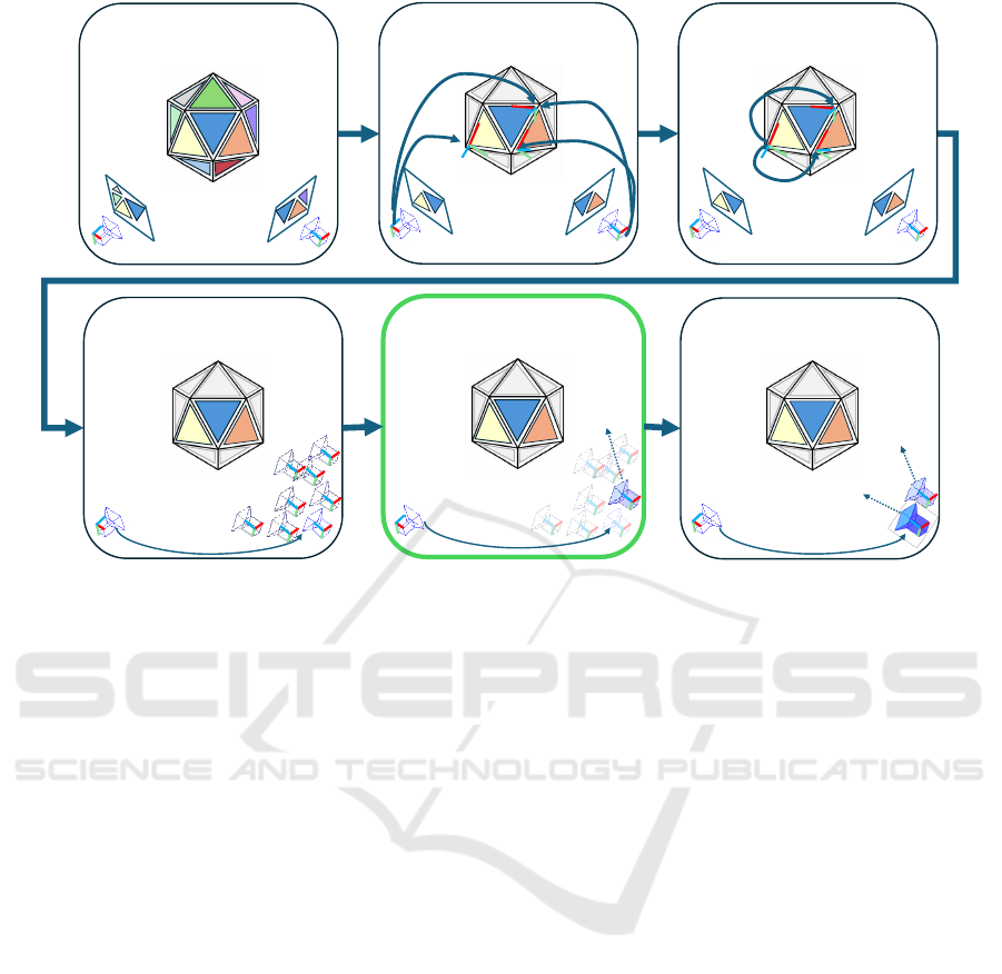
Step 1: Board Detection

& Intrinsic Calibration









Step 3: Estimation of

Board Parameters

































Step 5: Proposed Method to

Find the Best Initial Guess









Step 4: Initial Guesses for

Camera Extrinsic Parameters









Step 6: Bundle Adjustment to

Refine Extrinsic Parameters

Initial guess

Final Estimation







































Initial guess

Step 2: Board Pose Estimation

& Outlier Pose Rejection





















































































































Figure 1: The complete pipeline of PrIcosa consists of 6 steps. Step 1: Each board is uniquely identiﬁed by its distinct

ChArUco markers, and intrinsic parameters are calculated after detection. Step 2: Camera-to-board projection is calculated

using intrinsic parameters and views with large re-projection error are rejected. Step 3: Transformation from master board

to slave boards are calculated. Step 4: Initial guess of master camera to slave camera

′

is calculated for all possible

equations. Step 5: Probabilistic method is applied to select the best initial guess of

′

. Step 6: Reﬁnement of initial guess

and calculation of ﬁnal estimation is performed using bundle adjustment.

ﬁned set of views is then utilized to recalculate the

intrinsic parameters and distortion coefﬁcients. This

process of reﬁnement is performed iteratively, with

the recalculated parameters being obtained from the

ﬁltered subset of images. The iterations continue un-

til the level of error reaches a predeﬁned threshold of

improvement, essentially ensuring that the calibration

process converges to a stable solution.

2.2 Board Pose Estimation and Outlier

Rejection

Board pose estimation is the most crucial phase in

the multi-camera calibration process where the spatial

orientation and position of each camera in relation to

a calibrated reference board are determined. In this

step, we estimate the relative pose of all the cameras

for each observed board using the intrinsic parameters

that were calculated in the previous step. For esti-

mating the pose, we use the OpenCV implementation

of solvePnP iterative algorithm. In real-world scenar-

ios, noise and various factors can introduce errors in

the calibration process. To ensure the robustness and

reliability of the calibration results, we ﬁlter out the

poses that exhibit re-projection error beyond a certain

threshold of acceptance. These outlier poses are ex-

cluded from subsequent calibration steps.

2.3 Board Parameter Calculation

Our objective is to determine the relative poses be-

tween calibration boards to ultimately assemble them

into 3D objects. These 3D objects are composed of

multiple planar calibration boards. When a single im-

age captures two or more of these boards, it provides

an opportunity to estimate their relative poses, estab-

lishing pair-wise relationships. We collect measure-

ments from all images where pairs of boards are vis-

ible together and compute the average inter-board ro-

tation and translation. For this step, we followed the

procedure discussed in (Rameau et al., 2022).

2.4 Extrinsic Camera Parameter

Calculation

2.4.1 For Overlapping Cameras

When two cameras share an overlapping ﬁeld of view

such that they see the same calibration pattern, then

the process of determining the transformation be-

PrIcosa: High-Precision 3D Camera Calibration with Non-Overlapping Field of Views

803

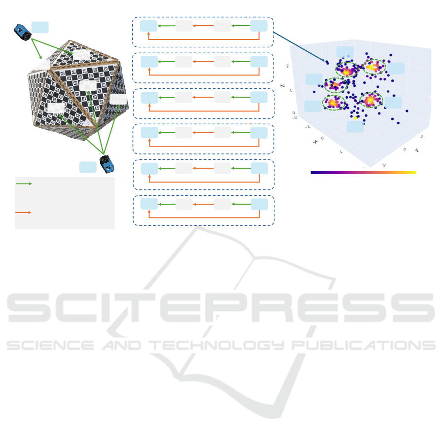
𝐵

a) Physical setup b) Connection graphs c) PDFs of transformations

Density

0 1

Known rigid 6DoF

transformation

Unknown rigid 6DoF

transformation

𝑐

(1)

(2)

(3)

(4)

(5)

(6)

𝑐

𝐵

𝑐

𝐵

Figure 2: The physical setup of the calibration system, shown in a) with only two of the six cameras, can be represented

by connection graphs, which can be seen in b) and correspond to 6DoF rigid transformations. Most of the time, there are

multiple paths to create a closed chain of transformations between two cameras. The selection of this chain, or connection

graph, affects the quality of the camera calibration signiﬁcantly. In c) every dot represents a camera position after choosing

one of the possible transformation chains. One probability density cluster for each of the six cameras is included in the

diagram. For each camera the transformation chain corresponding to the point in the cluster center is chosen to get the best

calibration results.

tween them becomes more straightforward. In this

particular phase, we have gathered all pairs of cam-

eras that possess a common ﬁeld of view, and subse-

quently, we have employed the OpenCV stereoCali-

brate method to compute their spatial relationship.

2.4.2 For Non-Overlapping Cameras

When cameras do not have overlapping ﬁelds of view,

meaning they are not capturing the same scene si-

multaneously, then more sophisticated approaches are

necessary. In such cases, traditional calibration meth-

ods that rely on shared scene points between cam-

eras are not directly applicable. To address this chal-

lenge, we employ a hand-eye calibration approach.

We designate one camera as the master (reference)

camera and the others as slave cameras. The calibra-

tion boards viewed by the master camera are termed

master boards, while those captured by slave cam-

eras are called slave boards. In Figure 2, we illustrate

a situation where the camera C

captures boards B

and B

, and another camera C

captures the boards

, B

, and B

. In this setup, C

serves as the mas-

ter camera with B

and B

as master boards, while

is a slave camera with B

, B

, and B

as its slave

boards. Each calibration group follows the sequence:

slave_camera → slave_board → master_board →

master_camera. This conﬁguration can be mathemat-

ically modeled using the equation AX = ZB, which

can be effectively solved using the hand-eye calibra-

tion method proposed by Tsai et al. (Tsai and Lenz,

1989).

However, it’s important to note that not all hand-

eye calibration groups have a diverse range of images

needed for accurate calibration. To address this limi-

tation, we have introduced an additional ﬁltering tech-

nique to exclude irrelevant poses from these groups.

Initially, we gather all possible one-to-one pose com-

binations for hand-eye calibration. Then, we analyze

the rotation vectors associated with these poses. If

there is any pose angle that signiﬁcantly deviates from

the others, the hand-eye calibration algorithm can en-

counter issues related to rotation normalization. To

address this issue, we have introduced a precaution-

ary measure to ﬁlter out problematic poses before

initiating the hand-eye calibration algorithm. In this

regard, we have employed the mean-shift clustering

algorithm (Carreira-Perpinán, 2015) to group similar

poses together. If any resulting cluster contains only

one pose element, we automatically discard that clus-

ter. Subsequently, we proceed to compute the hand-

eye calibration for the cameras with the remaining

poses.

VISAPP 2025 - 20th International Conference on Computer Vision Theory and Applications

804

2.4.3 Probabilistic Method for Outlier Rejection

When dealing with multiple planar calibration ob-

jects, a single camera can capture different boards in

various frames, which introduces complexity to the

calibration system.

For the particular situation observed in Figure 2,

we observe six calibration groups and derive the fol-

lowing six equations (1)-(6) to compute the transfor-

mation from the camera C

to the camera C

(

These equations result in six different

′

transfor-

mations. In an ideal setting, all six of these transfor-

mations would align perfectly. However, in practical

scenarios, this is not the case.

′

(1)

′

(2)

′

(3)

′

(4)

′

(5)

′

(6)

In the next step, we calculate the probability den-

sity function (PDF) of these six

′

transforma-

tions. Among these possibilities, we select the trans-

formation that exhibits the highest probability as our

initial estimate. For calculating PDF, we use the

Gaussian Kernel Density Estimation method (W˛eglar-

czyk, 2018). The process is explained in Algorithm

1. It is important to note that this step applies to both

non-overlapping and overlapping scenarios.

2.5 Bundle Adjustment

In this phase, we reﬁne all camera-to-camera and

board-to-board transformations to minimize the over-

all re-projection error using bundle adjustment. For

clarity, we denote the master camera as C

and slave

cameras as C

. The sets of master and slave boards

are represented as B

and B

, respectively.

We calculate the re-projection error for each of the

observed images. For instance, for pose ’p’ camera

observes board B

. For the same pose ’p’ master

camera C

observes board B

. Then we can calculate

the camera C

to board B

transformation as follows:

(7)

If camera C

(with intrinsic parameters K

) detects

N image points (x) on board B

at pose ’p’ and their

corresponding 3D points are X, the re-projection error

for that pose is:

Algorithm 1:

Calibration.

Input: Camera Intrinsics(2.1), Board Poses(2.2)

Output:

Total_Cameras ← C

, C

;

Total_Boards ← B

, B

;

Master_Camera ← C

;

Master_Boards ← B

, B

;

Slave_Boards ← B

, B

;

for B

in Master_Boards do

for B

in Slave_Boards do

←

cv2.calibrateRobotWorldHandEye(

);

rtmatrix ← Collect

;

tvecs ← Collect translation vectors from

;

end

density ← scipy.stats.gaussian_kde(tvecs);

max_idx ← argmax(density);

f inal

← rtmatrix[max _idx];

∑

i=1



− K



(8)

Similarly, we calculate the re-projection errors for

all the images of all the cameras and take the average

to calculate the overall re-projection error.

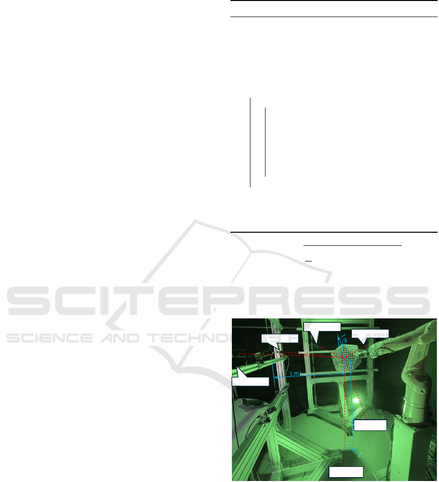
Cam-02

Cam-05

Cam-03

Cam-06

Cam-04

Cam-01

1 m

Figure 3: In our use case we have 6 cameras. The distance

between each consecutive camera is around 1 meter and the

distance between each camera pair baseline to the calibra-

tion object is also around 1 meter.

3 EVALUATION

We evaluate our results using two calibration objects:

an icosahedron and a cube. For both of the objects, we

use the same camera setup and robot gripper move-

PrIcosa: High-Precision 3D Camera Calibration with Non-Overlapping Field of Views

805

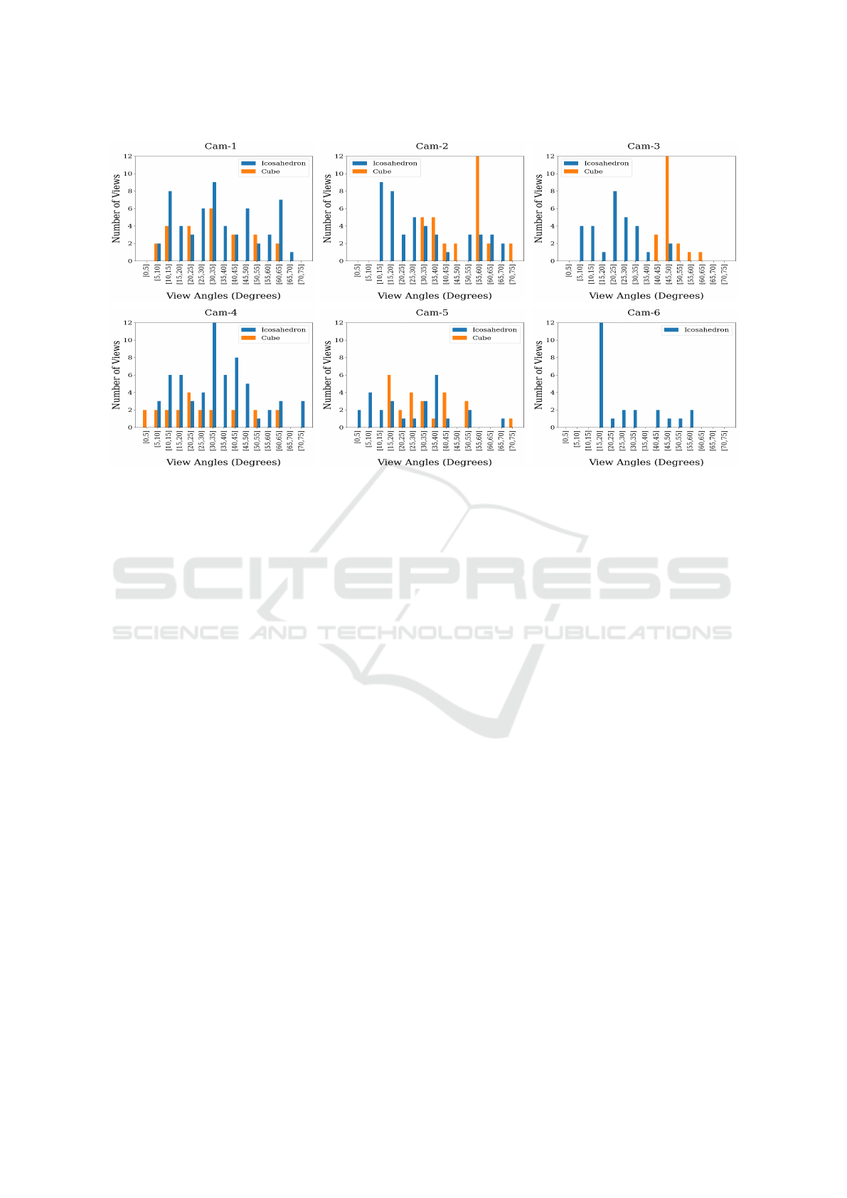
Figure 4: View angle variation for each camera. View angle is calculated from the camera to board projection matrix which

is derived from solvePnP algorithm. Then Euler angles (Roll, Pitch and Yaw) are calculated from that matrix. View angle =

∥Roll

+ Pitch

∥.

ments for image acquisition. In the following subsec-

tions, we compare the outcomes obtained from these

two calibration objects. We compare their differences

in the variation of the views, the coverage in the im-

age planes, and the resulting re-projection errors.

3.1 Experimental Setup

We utilize six 20MP monochrome industrial cam-

eras (DMK 33GX183 33G-Series from ’The Imaging

Source’) with 50 mm focal length. Each camera is

placed approximately 1 m away from the motion cen-

ter of the calibration object. The cameras are arranged

as stereo pairs with a baseline of 1 m. The camera

pairs each look at the calibration object from three

perpendicular directions, as shown in Figure 3.

The icosahedron is composed of equilateral trian-

gles with sides of 17 cm, and the cube has square faces

with sides of 220 cm. Both have the same ArUco

6x6_1000 pattern, where each square size is 13 mm.

To automatically move the calibration object to

different poses, we employ a Staubli TX2-60L robot.

The calibration object was mounted on the robot

gripper, and we used ROS1 Noetic (Open Source

Robotics Foundation, 2007) to control the robot and

MoveIt (Coleman et al., 2014) to plan the motions for

reaching the desired target poses with the calibration

object.

To move the object with the robot hand, we fol-

lowed a very simple motion plan. We moved the ob-

ject around the Z axis of the gripper by an Euler angle

of −280

◦

to 280

◦

. The dataset is available at (Nova

and Kedilioglu, 2024).

We adopted the "multical" (Batchelor, 2024)

GitHub repository as a baseline for our multi-camera

calibration system and implemented necessary mod-

iﬁcations to address the speciﬁc challenges of non-

overlapping camera setups.

3.2 View Variation

To achieve robust intrinsic parameter calibration, it

is essential to ensure a wide variety of views for all

the cameras. Optimal performance appears to be ob-

tained when the angle between the image plane and

the pattern plane is around 45° (Zhang, 1999). Re-

garding camera extrinsic parameter calibration, par-

ticularly with the hand-eye calibration method, it is

equally important to gather a large number of views

with signiﬁcant variation (Tsai and Lenz, 1989).

To calculate the angle between the image plane

and the pattern plane, we utilized the solvePnP algo-

rithm, which provides the transformation between the

camera and the board coordinates. This transforma-

tion results in a homogeneous matrix that we convert

into Euler form. This conversion yields three rota-

tion vectors: Roll, Pitch, and Yaw. Since the rotation

around the Z-axis (Yaw) shows limited variation in

pose, we exclude the yaw angle and instead focus on

the absolute values of the Roll and Pitch angles, which

VISAPP 2025 - 20th International Conference on Computer Vision Theory and Applications

806

Object Cam-1 Cam-2 Cam-3 Cam-4 Cam-5 Cam-6

Cube

Icosahedron

Figure 5: Image plane re-projection error after Bundle adjustment. It shows the average point error on a speciﬁc area of the

image plane.

we deﬁne as the ’view angle’. For other computer vi-

sion tasks the rotation around the optical axis (= Yaw)

is also not considered relevant (Mavrinac, 2012).

View angle = ∥Roll

+ Pitch

∥ (9)

The comparison between the two calibration ob-

jects concerning view angle variation is illustrated in

(Figure 4). Each bar in the plot represents the number

of views within a speciﬁc view angle range. The plot

clearly shows that images captured from the icosa-

hedron object exhibit greater pose variety than those

from the cube object. Additionally, it is noted that

camera-6 did not detect any points for the cube cali-

bration object, despite identical conditions for image

acquisition being maintained for both objects.

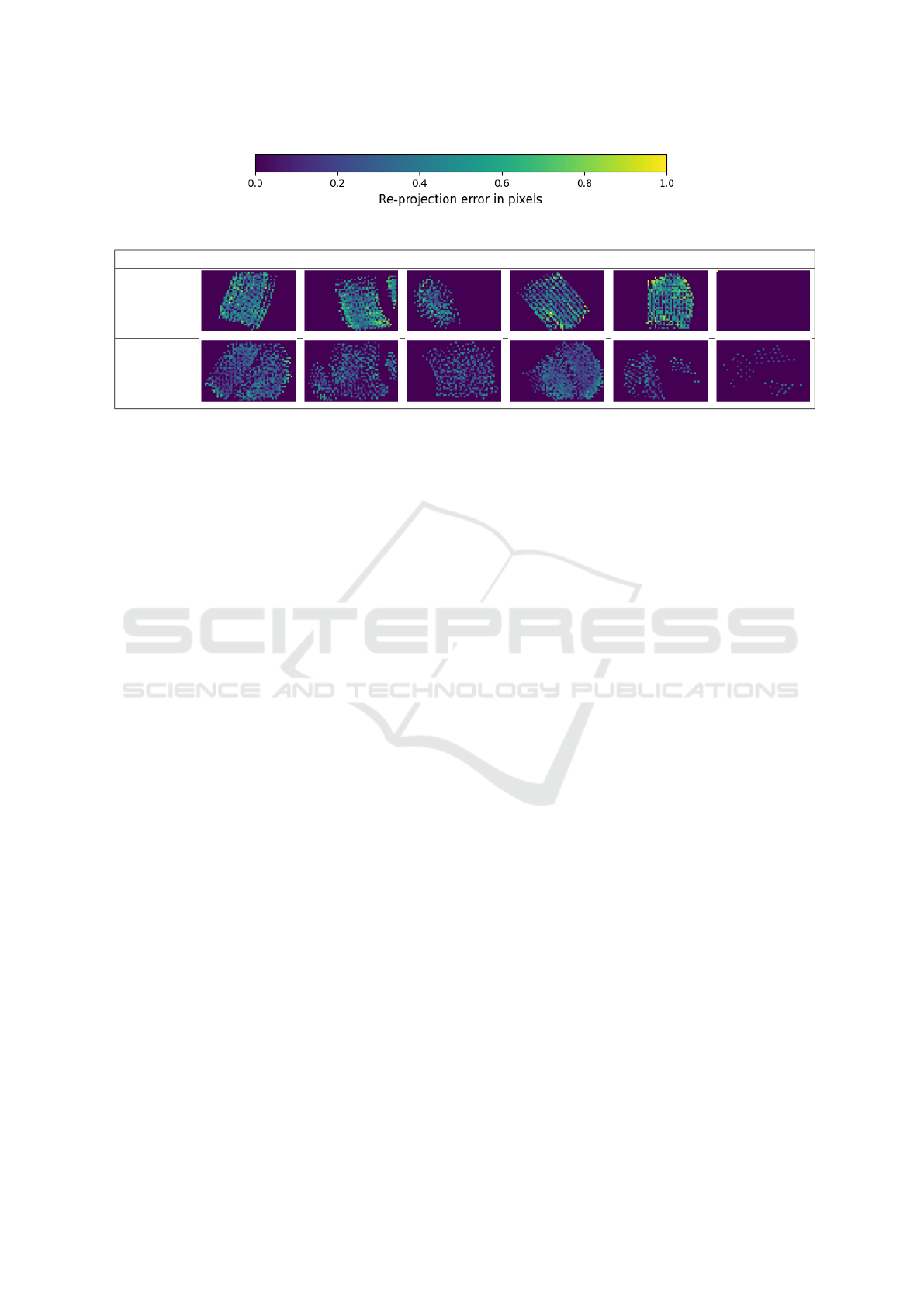
3.3 Coverage in Image Plane

Distortion mostly affects near the edges of the im-

age plane, so placing the calibration pattern near these

edges is crucial. Ensuring a wider coverage area al-

lows a more robust estimation of distortion parame-

ters.

Figure 5 shows a heat map of the re-projection er-

ror for all of the points present on the image plane

of each camera. This representation offers us a com-

prehensive insight into the extent of coverage of the

image plane.

The image clearly shows that the icosahedron ob-

ject achieves a larger coverage area with lower re-

projection error compared to the cube object.

3.4 Per View Re-Projection Error

Figure 6 displays the ﬁnal re-projection error re-

sults. In this experiment, 20 images from each cam-

era were captured using the same robot motion and

camera setup. Each bar in the graph represents the

re-projection error for an individual image. The re-

sults clearly indicate that for all cameras, the overall

re-projection error when using the icosahedron ob-

ject is consistently below 1 pixel. In contrast, the

cube calibration object results in signiﬁcantly higher

re-projection errors. This demonstrates the superior

accuracy and effectiveness of the icosahedron in cali-

brating the cameras.

3.5 Discussion

Throughout the experiments, we have highlighted the

importance of maintaining large variability in cam-

era poses for good-quality calibration. Figure 4 and

5 illustrate the superior coverage and view variation

achieved using the icosahedron compared to the cube,

and Figure 6 presents the resulting calibration results.

Despite the complexity of our camera setup, the

distinctive shape of the icosahedron enabled us to at-

tain the necessary view variety with minimal robot

motion. While it might be possible to replicate simi-

lar results with a cube, it would require more intricate

robot motions, which would need to be adjusted for

different camera setups. In industrial settings with an

increasing number of cameras, such adjustments be-

come increasingly challenging and time-consuming.

The icosahedron, therefore, offers an elegant and efﬁ-

cient solution, streamlining the calibration process in

complex, multi-camera environments.

Even after meeting all calibration criteria, it is

possible that sometimes the ﬁnal re-projection error

may still be high. This could occur if the bundle ad-

justment process converges at a local minimum. A

good initial guess can help prevent this issue, and

our probabilistic algorithm assists in selecting opti-

mal initial guesses. During the extrinsic parameter

PrIcosa: High-Precision 3D Camera Calibration with Non-Overlapping Field of Views

807

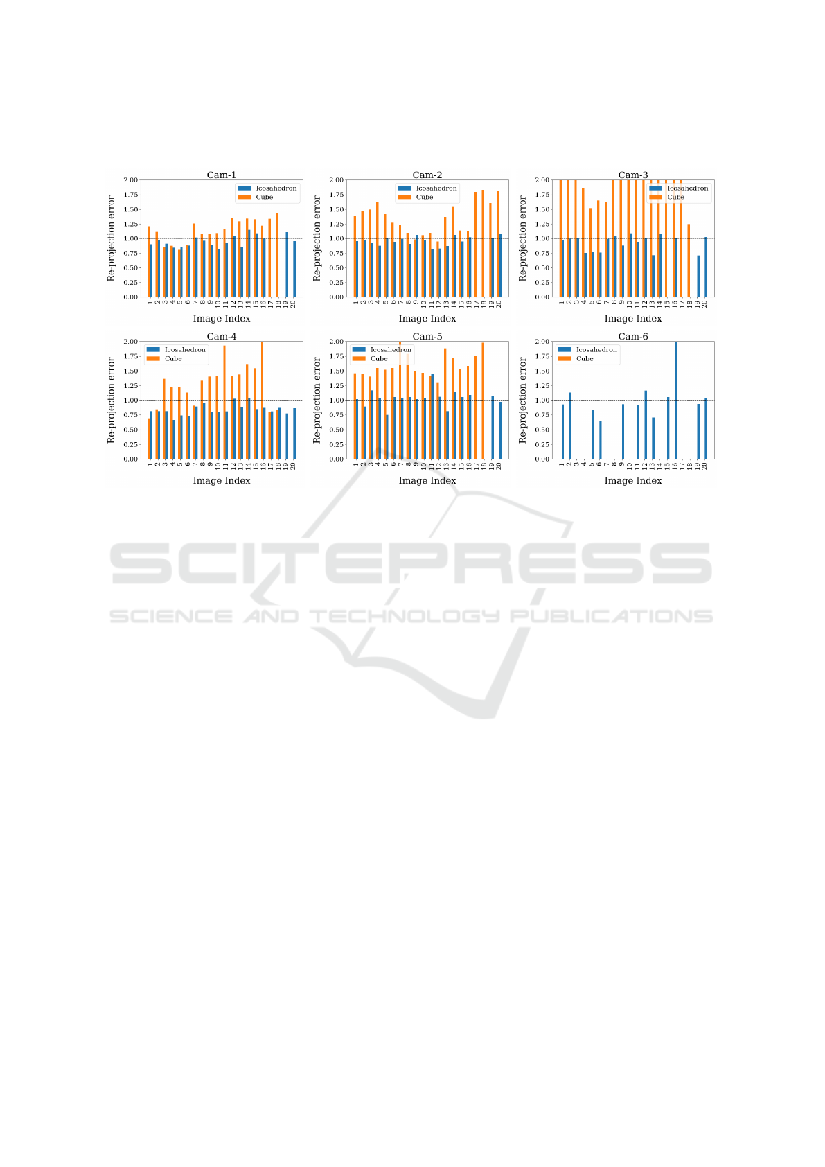
Figure 6: Per image re-projection error after bundle adjustment. One image consists of multiple views. Image re-projection

error is the average error of all views.

calibration, we observed that some calibration groups

were highly scattered. This scattering tends to occur

when a group has fewer images, limited variety, or

incorrect pose estimations. When using a calibration

object with a large number of boards, it becomes pos-

sible to create a large number of calibration groups,

which facilitates a more robust initial guess. For in-

stance, with the icosahedron object, we have around

100 groups for each camera pair. While some groups

are outliers, the inlier groups tend to cluster densely

around the center (Figure 2(c)), aiding in the selection

of initial parameters. In contrast, using the cube ob-

ject results in an average of only 4 groups per camera,

making it challenging to estimate a robust solution.

The structural advantage of the icosahedron, com-

bined with the probabilistic approach of our PrIcosa

framework, enables it to identify the optimal calibra-

tion group even from subpar datasets. For instance,

when analyzing the icosahedron datasets from cam-

eras 5 and 6, we observe that these cameras have lim-

ited view variation and image plane coverage (Figure

4 and 5). Despite these shortcomings, our framework

still manages to ﬁnd the best solution within the poor

dataset (Figure 6).

4 CONCLUSIONS

We have shown that an icosahedron-shaped calibra-

tion object leads to considerably better calibration re-

sults than a cube-shaped calibration object for the

same set of views and calibration object poses. The

icosahedron represents a better balance between the

quantity and size of the boards. It provides signif-

icantly more variety in the dataset and better cover-

age of the image planes with useful patterns. This en-

ables smaller re-projection error values and improves

the calibration accuracy.

To get the most out of the acquired dataset, we

developed and evaluated a probabilistic method that

uses an optimized subset of possible input equations

for the optimization algorithms that are used to cal-

ibrate the cameras. By taking the cluster center of

all possible camera positions generated by the prob-

ability density function, we can minimize the re-

projection error in the calibration process.

Further research could consist of the exploration

of different calibration patterns. The localization of

the features of these patterns should be accurate and

robust. The patterns should also work in the case of

partial overlap. They should have a unique ID such

that each board can be identiﬁed in the images. Their

geometry should be able to handle sharp angles and

still be accurate enough. This would allow to increase

VISAPP 2025 - 20th International Conference on Computer Vision Theory and Applications

808

the pose variety in the dataset.

Another aspect that deserves further investigation

is the selection of the reference camera. Our cur-

rent implementation is time-consuming, mainly in the

bundle adjustment phase. This process involves se-

lecting each camera as the reference camera in turn

and performing the bundle adjustment repeatedly, re-

sulting in increased time requirements as the number

of cameras grows. A potential modiﬁcation to address

this issue involves dynamically selecting the best ref-

erence camera by analyzing the observed views of

each camera. Our evaluation in the previous sec-

tion demonstrated that cameras with a substantial de-

gree of pose variability yield better results. There-

fore, automatically determining the reference camera

based on observed view characteristics could opti-

mize the calibration process, especially in scenarios

with a large number of cameras.

ACKNOWLEDGEMENTS

The project received funding from the German Fed-

eral Ministry of Education and Research under grant

agreement 05K22WEA / 05K22WO1 (AutoTron).

REFERENCES

Abedi, F., Yang, Y., and Liu, Q. (2018). Group geometric

calibration and rectiﬁcation for circular multi-camera

imaging system. Opt. Express, 26(23):30596–30613.

An, G. H., Lee, S., Seo, M.-W., Yun, K., Cheong, W.-S., and

Kang, S.-J. (2018). Charuco board-based omnidirec-

tional camera calibration method. Electronics, 7(12).

Batchelor, O. (2024). multical. https://github.com/

oliver-batchelor/multical. GitHub repository.

Bradski, G. (2000). The opencv library. Dr. Dobb’s Jour-

nal: Software Tools for the Professional Programmer,

25(11):120–123.

Carreira-Perpinán, M. A. (2015). A review of mean-

shift algorithms for clustering. arXiv preprint

arXiv:1503.00687.

Coleman, D., Sucan, I., Chitta, S., and Correll, N. (2014).

Reducing the barrier to entry of complex robotic

software: a moveit! case study. arXiv preprint

arXiv:1404.3785.

D’Emilia, G. and Di Gasbarro, D. (2017). Review of tech-

niques for 2d camera calibration suitable for industrial

vision systems. In Journal of Physics: Conference Se-

ries, volume 841, page 012030. IOP Publishing.

Ha, H., Perdoch, M., Alismail, H., Kweon, I. S., and

Sheikh, Y. (2017). Deltille grids for geometric camera

calibration. In 2017 IEEE International Conference

on Computer Vision (ICCV), pages 5354–5362.

Li, B., Heng, L., Koser, K., and Pollefeys, M. (2013).

A multiple-camera system calibration toolbox using

a feature descriptor-based calibration pattern. In

2013 IEEE/RSJ International Conference on Intelli-

gent Robots and Systems, pages 1301–1307.

Lv, Y., Feng, J., Li, Z., Liu, W., and Cao, J. (2015). A new

robust 2d camera calibration method using ransac.

Optik, 126(24):4910–4915.

Mavrinac, A. (2012). Modeling and optimizing the cover-

age of multi-camera systems.

Nova, T. T. (2024). Pricosa: High-precision 3d

camera calibration with non-overlapping ﬁeld of

views. https://github.com/TabassumNova/Multi_

Camera_Calibration. GitHub repository.

Nova, T. T. and Kedilioglu, O. (2024). Non-Overlapping

Multi-Camera Calibration Dataset using Icosahedron

and Cube Calibration Object. https://doi.org/10.5281/

zenodo.13294455.

Open Source Robotics Foundation (2007). Robot operating

system (ros). https://www.ros.org. https://www.ros.

org.

Oš

cádal, P., Heczko, D., Vysocký, A., Mlotek, J., Novák,

P., Virgala, I., Sukop, M., and Bobovský, Z. (2020).

Improved pose estimation of aruco tags using a novel

3d placement strategy. Sensors, 20(17).

Rameau, F., Park, J., Bailo, O., and Kweon, I. S. (2022).

Mc-calib: A generic and robust calibration toolbox for

multi-camera systems. Computer Vision and Image

Understanding, 217:103353.

Tabb, A. and Medeiros, H. (2019). Calibration of asyn-

chronous camera networks for object reconstruction

tasks. CoRR, abs/1903.06811.

Tsai, R. and Lenz, R. (1989). A new technique for fully au-

tonomous and efﬁcient 3d robotics hand/eye calibra-

tion. IEEE Transactions on Robotics and Automation,

5(3):345–358.

W˛eglarczyk, S. (2018). Kernel density estimation and its

application. In ITM web of conferences, volume 23,

page 00037. EDP Sciences.

Zhang, Z. (1999). Flexible camera calibration by viewing a

plane from unknown orientations. In Proceedings of

the Seventh IEEE International Conference on Com-

puter Vision, volume 1, pages 666–673 vol.1.

Zhang, Z. (2000). A ﬂexible new technique for camera cal-

ibration. IEEE Transactions on Pattern Analysis and

Machine Intelligence, 22(11):1330–1334.

PrIcosa: High-Precision 3D Camera Calibration with Non-Overlapping Field of Views

809