Robust Autocorrelation for Period Detection in Time Series

Zhi Yang, Likun Hou and Xing Zhao

SAP HANA, SAP Labs China, 1001 Chenghui Road, Shanghai, China

{zhi.yang, likun.hou, brook.zhao}@sap.com

Keywords:

Robust Autocorrelation, MAD Filter, Period Detection, Time Series, Outlier.

Abstract:

Autocorrelation is a key tool in time series period detection, but its sensitivity to outliers is a signiﬁcant

limitation. This paper introduces a robust autocorrelation method for period detection that minimizes the

inﬂuence of outliers. By incorporating a moving average and applying a Median Absolute Deviation (MAD)

ﬁlter to each cycle-subseries, we signiﬁcantly enhance the robustness of the autocorrelation to outliers. The

MAD ﬁlter identiﬁes and corrects outliers in the cycle-subseries, based on the assumption that the cycle-

subseries consists of a constant plus Gaussian noise. This innovative robust autocorrelation can effectively

replace traditional autocorrelation in existing period detection algorithms. Additionally, we propose a new

algorithm that leverages our robust autocorrelation. Both theoretical analysis and empirical tests on real-world

and synthetic datasets indicate that period detection algorithms using our proposed robust autocorrelation

outperform those using traditional autocorrelation. Furthermore, our proposed algorithm surpasses all other

existing algorithms in comparison.

1 INTRODUCTION

A time series is considered periodic if a certain pattern

repeats at regular intervals of time. Periodicity can

occur due to natural phenomena, such as changes in

temperature or seasonal ﬂuctuations in product sales,

or due to human activities, such as electricity usage

or trafﬁc ﬂows. The causes of periodicity are often

clear, and the periods are typically daily, weekly or

yearly. However, there are also many time series that

are related to other phenomena, and detecting peri-

odicity can be challenging, particularly when there is

limited information available. Nevertheless, the abil-

ity to identify the period of a time series is essential

for data analysis and forecasting.

In real-world datasets, outliers are a common oc-

currence. In time series data, an outlier is a data point

that deviates signiﬁcantly from the general behavior

of the remaining data points. Outliers can have var-

ious causes, including data entry errors, experimen-

tal errors, sampling errors, and natural outliers. They

can signiﬁcantly impact the results of data analysis

and forecasting, such as period detection. Outliers

can affect traditional autocorrelation and, therefore,

inﬂuence the detection of periods. Inaccurate period

detection of time series can result from outliers.

The existing period detection algorithms of time

series can be classiﬁed into three groups:1) frequency

domain methods that rely on the periodogram af-

ter Fourier transform, such as Hyndman’s ﬁndfre-

quency (Hyndman, 2023), Fisher’s test (Fisher, 1929;

Wichert et al., 2004) and Lomb-Scargle (Hu et al.,

2014; Glynn et al., 2006; Lomb, 1976); 2) time do-

main methods that rely on autocorrelation function

(ACF), such as seasonality test in Predictive Analy-

sis Library (PAL) of SAP HANA (SAP, 2024), me-

dian distance of autocorrelation function peaks (ACF-

Med) as well as methods proposed in (Wang et al.,

2005; Breitenbach et al., 2023); 3) methods that com-

bine periodogram and autocorrelation, such as AU-

TOPERIOD (Vlachos et al., 2005; Puech et al., 2020),

SAZED (Toller et al., 2019) and methods proposed

in (Parthasarathy et al., 2006; Wen et al., 2023; Wen

et al., 2021). However, most of these algorithms are

not robust to outliers. The algorithms presented in

(Wen et al., 2023; Wen et al., 2021) claim to be ro-

bust to outliers, and we will include their results in

the comparison.

In this work, we propose a novel autocorrelation

method that demonstrates high robustness to outliers,

thereby enhancing the reliability of period detection

algorithms. For every lag h, we detrend the time series

using a moving avarage with window size h, followed

by the application of a Median Absolute Deviation

(MAD) ﬁlter on each cycle-subseries to identify and

correct outliers. The MAD ﬁlter, a non-local ﬁlter,

Yang, Z., Hou, L. and Zhao, X.

Robust Autocorrelation for Period Detection in Time Series.

DOI: 10.5220/0013092500003890

Paper published under CC license (CC BY-NC-ND 4.0)

In Proceedings of the 17th International Conference on Agents and Artiﬁcial Intelligence (ICAART 2025) - Volume 2, pages 36-44

ISBN: 978-989-758-737-5; ISSN: 2184-433X

detects and adjusts datapoints in the cycle-subseries

that fall outside the range of 3 MAD. Our proposed

autocorrelation method can effectively replace tradi-

tional autocorrelation techniques used in period de-

tection algorithms, signiﬁcantly enhancing their re-

silience to outliers. This improvement beneﬁts algo-

rithms such as ACF-Med, AUTOPERIOD, SAZED,

and PAL’s seasonality test. Furthermore, we present

a novel algorithm that utilizes the proposed autocor-

relation, showcasing superior performance compared

to the aforementioned algorithms. Our approach in-

volves performing peak analysis on the proposed au-

tocorrelation. Although the source code for the algo-

rithms introduced in (Wen et al., 2023; Wen et al.,

2021) is not publicly available, our new algorithm

achieves better results than those reported in (Wen

et al., 2023; Wen et al., 2021) when evaluated on the

CRAN dataset (Hyndman and Killick, 2023), despite

the previous algorithms also claiming robustness to

outliers.

Robust period detection plays a vital role in many

real-world applications. One such application is the

decomposition of time series with unknown peri-

ods using robust methods like STL (Cleveland et al.,

1990), where robust period detection is essential. Ad-

ditionally, in the context of time series outlier detec-

tion discussed in (Gao et al., 2020), robust period de-

tection serves as an indispensable step. Numerous

other applications that involve robust period detection

can be found in (Tolas et al., 2021; Zhang et al., 2022;

Wang et al., 2006; Vlachos et al., 2004).

The remainder of this paper is organized as fol-

lows: Section 2 delves into a detailed discussion of

the proposed autocorrelation and provides an illustra-

tive example. In Section 3, we present the experimen-

tal results obtained from public algorithms, where tra-

ditional autocorrelation has been substituted with pro-

posed autocorrelation. Section 4 introduces our novel

period detection algorithm and discusses the corre-

sponding experiments and ablation studies. Finally,

our conclusions are presented in Section 5.

To facilitate readers of interest, we summarize a

list of abbreviations which are frequently used in this

paper in Table 1.

2 PROPOSED

AUTOCORRELATION

2.1 Proposed ACF Formula

Autocorrelation is a fundamental tool used to de-

tect the period of a time series. Given a time series

x = {x

|i = 0,1,··· ,N − 1} with N data points, the

Table 1: List of Abbreviations.

Abbreviation Description

M-MA ACF

ACF of time series detrended by moving average and ﬁl-

tered by MAD ﬁlter on every cycle-subseries.

MA ACF ACF of time series detrended by moving average

M-RAW ACF ACF of original time series ﬁltered by MAD ﬁlter on every

cycle-subseries.

RAW ACF ACF of original time series

LPA left peak analysis

ACF-LPA left peak analysis on ACF

X ACF-LPA left peak analysis on X ACF. X can be M-MA, MA, M-

RAW and RAW.

autocorrelation function (ACF) of lag h is deﬁned as:

= c

, (1)

where c

is the autocovariance function at lag h. The

deﬁnition of c

N−h−1

∑

t=0

− ¯x)(x

t+h

− ¯x), (2)

where ¯x is the mean of the time series. The value of γ

is in the range of -1 to 1, with a larger value indicating

more relevance. For a time series with N elements, γ

is deﬁned with h = 0, 1, · · · ,N − 1.

To address the limitation of the above traditional

ACF’s sensitivity to outliers, we propose a robust

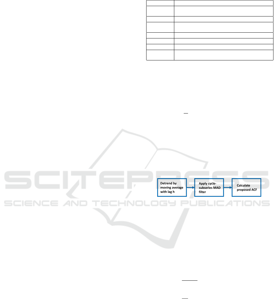
ACF, as illustrated in Figure 1.

Figure 1: The process for computing proposed ACF.

The ﬁrst step involves obtaining the detrended

time series through a moving average. Similar to

the weighted moving average discussed in (Hyndman,

2018) and the moving average used in PAL’s seasonal-

ity test (SAP, 2024), the trend time series m

is deter-

mined by taking the moving average of window size

h for a given time series x

x and lag h, as shown in (3)

and (4),











2q + 1

∑

j=−q

i+ j

, h = 2q + 1

, h = 2q

(3)

= 0.5x

i−q

q−1

∑

j=−q+1

i+ j

+ 0.5x

i+q

(4)

where i = 0,1,··· ,N −1. In (3) and (4), if i−q < 0 or

i + j < 0, x

i−q

or x

i+ j

is replaced by x

. Conversely, if

i + q > N −1 or i+ j > N −1, x

i+q

or x

i+ j

is replaced

by x

N−1

. This ensures the trend time series m

retains

the length N. The detrended time series y

is then

obtained by y

= x

x − m

Robust Autocorrelation for Period Detection in Time Series

It is important to note that the window size must

be the same as the lag at this step. When the actual

period is the same as the lag h in this case, the pe-

riodicity is reinforced after removing the trend using

the moving average. However, if h is smaller than the

actual period, the periodicity of the detrended time

series is reduced, resulting in a low ACF for lag h.

When h is a little larger than the actual period, the

seasonal part is also emphasized in the detrended time

series. Nonetheless, the ACF for lag h is lower than

the ACF of the actual period due to the ACF formula

(1) and (2). As the lag h increases, more of the trend

component is included in the detrended time series.

The second step involves the cycle-subseries

MAD ﬁlter in the detrended time series y

. The MAD

ﬁlter is a non-local ﬁlter based on MAD method. It

detects and adjusts datapoints in the cycle-subseries

that fall outside the range of 3 MAD. It is inspired

by the cycle-subseries smoothing and ﬁltering proce-

dures in STL decomposition (Cleveland et al., 1990)

and the non-local means algorithm used in image

denoising (Buades et al., 2005). For each lag h,

we generate h cycle-subseries. Given the i-th cycle-

subseries z

i,h

= {y

i+kh

|k ≥ 0, i + kh < N}, we denote

i,h

= y

i+kh

. Let

ˆz

i,h

= median(z

i,h

) (5)

i,h

= |z

i,h

− ˆz

i,h

|, (6)

mad

i,h

= median(d

i,h

). (7)

Then, we calculate the MAD score of each point in

i,h

. The MAD score is deﬁned as follows:

i,h

= 0.67449 ·

i,h

− ˆz

i,h

mad

i,h

. (8)

The coefﬁcient 0.67449 is used to make the MAD

score equivalent to the Z score when the data follows

a Gaussian distribution. After applying the MAD ﬁl-

ter, the ﬁltered cycle-subseries is as follows:

˜z

i,h











ˆz

i,h

− 3/0.67449 · mad

i,h

, s

i,h

< −3

i,h

, −3 ≤ s

i,h

≤ 3

ˆz

i,h

+ 3/0.67449 · mad

i,h

, s

i,h

> 3

(9)

Let us put the cycle-subseries back to the whole

time series. After applying the cycle-subseries MAD

ﬁlter to all cycle-subseries, we get the ﬁltered whole

time series

as ˜y

i+kh

= ˜z

i,h

This approach involves outlier detection using the

MAD score, detecting and correcting outliers accord-

ing to the 3 MAD rule. We assume that the seasonal

component satisﬁes S

= S

i+T

. When the lag h is the

actual period or the integer multiples of the actual pe-

riod, the cycle-subseries satisfy z

i,h

= a

i,h

+ ε

, where

follows a Gaussian distribution with zero mean,

and a

i,h

is a constant. In this scenario, the MAD

ﬁlter can accurately detect outliers within the cycle-

subseries. The 3 MAD rule effectively detects and

corrects these outliers, thereby making the ACF ro-

bust to outliers.

When the lag h is neither the actual period nor

an integer multiple of the actual period, the cycle-

subseries do not satisfy z

i,h

= a

i,h

+ε

. Consequently,

the effectiveness of outlier detection and correction is

diminished compared to the previous case. This re-

sults in a smaller increase in the ACF than when the

lag h aligns with the actual period or its integer mul-

tiples.

The ﬁnal step involves calculating the proposed

ACF using the time series after detrending and ap-

plying the cycle-subseries MAD ﬁlter, denoted as

Similar to the traditional ACF, the proposed ACF at

lag h is deﬁned as

= ˜c

/ ˜c

, where ˜c

˜c

N−h−1

∑

i=0

( ˜y

− ˜y

)( ˜y

i+h

− ˜y

), (10)

where ˜y

is the mean of the detrended time series

The complexity of calculating the proposed ACF for

each lag is O(N), leading to a total complexity of

O(N

) if the number of lags for autocorrelation scales

with N. It’s worth noting that the proposed ACFs

across different lags can be computed in parallel.

2.2 An Illustrative Example

In this subsection, we will evaluate the proposed ro-

bust ACF with cycle-subseries MAD ﬁlter using a

simple case. To assess its robustness to outliers and

perform an ablation study, we construct four types of

ACFs based on the procedures outlined in Figure 1.

The proposed robust ACF depicted there is referred to

as M-MA ACF. If we omit the detrending process and

apply the cycle-subseries MAD ﬁlter on the original

time series, this version of ACF is termed M-RAW

ACF. When MAD ﬁlter is removed and the ACF is

calculated from the detrended time series, it is called

MA ACF. Finally, if both detrending and MAD ﬁlter

are removed, and the ACF is computed using the orig-

inal time series, we refer to it as RAW ACF. For our

analysis, we employ motion data from CRAN dataset

(Hyndman and Killick, 2023), which is monthly and

has a period of 12, with a total length of 192. This

data is illustrated in Figure 2a. The four ACFs of the

motion data, with lags ranging from 2 to 96, are pre-

sented in Figure 3a. It is evident that both M-MA

ACF and MA ACF exhibit a strong periodicity of 12.

M-RAW ACF and RAW ACF, however, show a de-

clining trend and reach maximum ACF at lag = 2,

ICAART 2025 - 17th International Conference on Agents and Artiﬁcial Intelligence

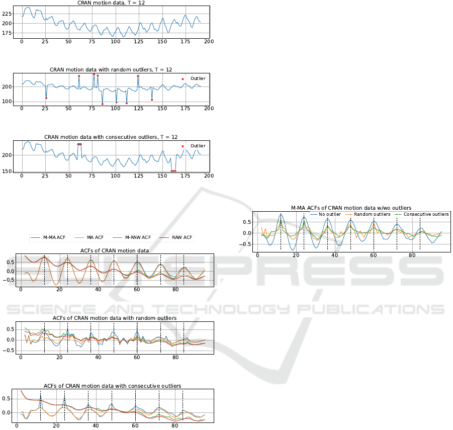
rather than 12. This occurs due to the presence of

a trend in the motion data and the absence of the de-

trending process in M-RAW ACF and RAW ACF.

(a) CRAN motion data, T = 12

(b) CRAN motion data with 9 random outliers, T = 12

Figure 2: CRAN motion data without outlier, with random

outliers and with consecutive outliers.

(a) ACFs of CRAN motion data without outlier

(b) ACFs of CRAN motion data with 9 random outliers

Figure 3: ACFs of CRAN motion data without outlier, with

random outliers and with consecutive outliers.

Now let us introduce random outliers into the mo-

tion data. We insert 9 outliers with an amplitude ﬁve

times the standard deviation of the original time se-

ries. The corresponding outlier ratio is 0.05. The

outlier-infused motion data is displayed in Figure 2b.

The four ACFs of outlier-infused motion data are de-

picted in Figure 3b. It’s evident that the M-MA ACF

retains a strong periodicity of 12. For other ACFs, the

periodicity of 12 is not obvious.

One might question the apparent outliers in Figure

2b, suggesting that local smoothing or range detection

algorithms could easily identify them. Let’s now con-

sider consecutive outliers in the motion data, which

prove more challenging to detect. Figure 2c shows

motion data with these consecutive outliers, nine in

total, divided into two sections. The four ACFs of

motion data with consecutive outliers are depicted in

Figure 3c. The periodicity of 12 remains evident in

the M-MA ACF and MA ACF. However, the values

of the MA ACF are signiﬁcantly reduced, peaking at

less than 0.2, with the maximum value taken at a lag

of 24 rather than 12. This periodicity of 12 becomes

less clear in the M-RAW ACF and RAW ACF.

Let’s now compare the M-MA ACFs of motion

data with and without outliers, as depicted in Figure

4. We observe that all instances exhibit a strong pe-

riodicity of 12, with comparable peak values. This

analysis demonstrates the robustness of M-MA ACFs

to outliers, including random, consecutive, and hard-

to-detect outliers.

Figure 4: M-MA ACF of CRAN motion data without out-

lier, with random outliers and with consecutive outliers.

3 EXPERIMENTS ON PUBLIC

ALGORITHMS WITH

PROPOSED ACF

3.1 Algorithms and Datasets

We explore period detection algorithms utilizing ACF,

substituting it with the four ACFs detailed in Section

2.2. These algorithms include PAL’s seasonality test,

ACF-Med, AUTOPERIOD, and SAZED. The origi-

nal ACF in SAZED is a 10-fold autocorrelation, as

outlined in (Toller et al., 2020).

PAL’s seasonality test computes the ACF from lag

= 2 up to half the series length, selecting the max-

imum ACF value. If this maximum ACF exceeds

the threshold (default is 0.2, which we use in sub-

sequent sections), the corresponding lag is consid-

ered as the period. If not, the series is deemed non-

periodic. We utilize the AUTOPERIOD implemen-

tation from (Schmidl, 2023) and the SAZED imple-

mentation from (Toller et al., 2020) in R studio.

For our datasets, we use the publicly available,

single-period time series data from CRAN, also ref-

Robust Autocorrelation for Period Detection in Time Series

erenced in (Toller et al., 2019). This data, sourced

from the “Time Series Data” section of “CRAN Task

View: Time Series Analysis” (Hyndman and Killick,

2023), comprises 82 time series, each labeled with its

corresponding period. Series lengths vary from 16 to

3024, with periods ranging from 2 to 52. Figure 2a

shows a time series from the CRAN dataset.

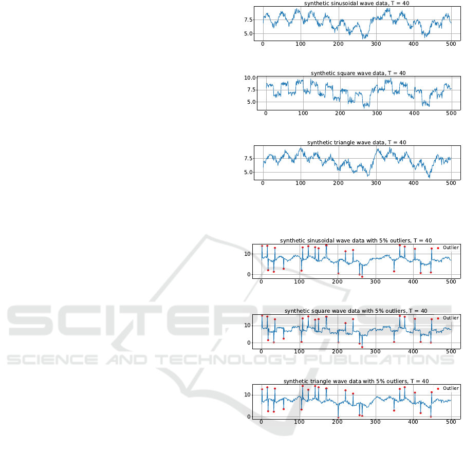
In addition, we generate 3000 synthetic time se-

ries, each of length 500, without outliers. Each se-

ries includes a piecewise linear trend, additive white

Gaussian noise (variance = 0.1), and a periodic com-

ponent with amplitude 1 and period between 10 to

50. We explore three periodic patterns: sinusoidal,

square, and triangular waves, with each pattern rep-

resented in 1000 series. Figure 5 shows examples of

sine wave data, square wave data, and triangle wave

data, all without outliers.

We also introduce outliers to both the CRAN and

synthetic datasets, with an amplitude ﬁve times the

standard deviation of the original time series. In (Wen

et al., 2023), the same outlier amplitude was also em-

ployed. For most real-world examples, an outlier that

exceeds ﬁve times the standard deviation is consid-

ered sufﬁciently large. Large outliers have a signiﬁ-

cant impact on periodicity detection. We aim to evalu-

ate the performance of the proposed ACF in handling

data with large outliers, as well as normal data. We set

the outlier ratio (OR) at 0.01, 0.03, or 0.05. Like (Wen

et al., 2023), since the outlier ratio is usually small in

real world, we limit the outlier ratio to a maximum of

0.05. For instance, the motion data depicted in Figure

2b with an OR of 0.05 represents a CRAN time series

with outliers. Similarly, Figure 6 illustrates examples

of sine wave data, square wave data, and triangle wave

data, each containing 5% outliers.

3.2 Experimental Results

Similar to (Wen et al., 2023; Wen et al., 2021), the

precision of every algorithm is calculated by the ratio

of the number of time series with correctly estimated

period length to the total number of time series. Ta-

ble 2 presents results from various algorithms based

on ACFs, applied to the CRAN dataset. For the un-

modiﬁed CRAN dataset, M-MA ACF and MA ACF

demonstrate comparable performance. However, in

the presence of outliers, M-MA ACF surpasses other

ACFs in algorithms PAL’s seasonality test, ACF-Med,

and SAZED. For AUTOPERIOD, the performances

of the four ACFs are similar, due to the reliance on pe-

riod hints provided by the periodogram method. This

method, however, underperforms due to the complex

trend in the CRAN dataset.

For the synthetic datasets, the ﬁndings are out-

(a) An example of synthetic sinusoidal wave data, T = 40

(b) An example of synthetic square wave data, T = 40

Figure 5: Examples of synthetic wave data, from top to bot-

tom are sinusoidal wave, square wave, and triangle wave.

(a) An example of synthetic sinusoidal wave data with 5% outliers, T = 40

(b) An example of synthetic square wave data with 5% outliers, T = 40

Figure 6: Examples of synthetic wave data with with 5%

outliers, from top to bottom are sinusoidal wave, square

wave, and triangle wave.

lined in Table 3, mirroring those from the CRAN

dataset. Without outliers, M-MA ACF and MA ACF

show similar performance. However, in the pres-

ence of outliers, M-MA ACF surpasses other ACFs

across all four algorithms, including AUTOPERIOD.

This superior performance is attributed to the piece-

wise linear trend in synthetic data, which is sim-

pler than CRAN, enabling the periodogram method

in AUTOPERIOD to perform better.

From our experiments on the CRAN and synthetic

datasets, we observed superior or equivalent perfor-

mance of M-MA ACF compared to other ACFs across

all tested algorithms. M-MA ACF signiﬁcantly out-

ICAART 2025 - 17th International Conference on Agents and Artiﬁcial Intelligence

Table 2: Precision of public algorithms on CRAN dataset.

The best results among ACFs are highlighted in bold.

Algorithms ACFs OR = 0 OR = 0.01 OR = 0.03 OR = 0.05

PAL

RAW 0.415 0.390 0.402 0.232

M-RAW 0.402 0.402 0.378 0.341

MA 0.768 0.537 0.329 0.195

M-MA 0.805 0.793 0.634 0.500

ACF-Med

RAW 0.451 0.402 0.183 0.012

M-RAW 0.451 0.366 0.317 0.220

MA 0.671 0.354 0.085 0.012

M-MA 0.671 0.646 0.524 0.402

AUTOPERIOD

RAW 0.451 0.366 0.293 0.207

M-RAW 0.415 0.354 0.305 0.220

MA 0.439 0.354 0.305 0.183

M-MA 0.451 0.390 0.317 0.256

SAZED

10-fold 0.549 0.500 0.439 0.415

RAW 0.524 0.512 0.463 0.390

M-RAW 0.524 0.488 0.500 0.427

MA 0.598 0.537 0.476 0.439

M-MA 0.585 0.537 0.488 0.488

performs other ACFs in the presence of outliers, with

its advantage becoming increasingly apparent as the

number of outliers increases. M-MA ACF can en-

hance the performance of existing algorithms.

Based on our experiments, we observed that the

PAL with M-MA ACF performs exceptionally well

when the outlier ratio is either 0 or 0.01. However,

its performance degrades at outlier ratios of 0.03 or

0.05. We also noticed that the PAL with M-MA ACF

detects periods in the time series as integer multiples

of the actual period in certain instances. For instance,

a time series with a period of 12 might be identiﬁed

as having a period of 24. In the case of the CRAN

dataset, if we accept these integer multiples as correct

detections, the precision is 0.841, 0.854, 0.744, and

0.695 for outlier ratios of 0, 0.01, 0.03, and 0.05, re-

spectively. We will leverage this property to propose

a new algorithm in the following section.

4 PROPOSED PERIOD

DETECTION ALGORITHM

4.1 Algorithm Description

In PAL’s seasonality test, the period is identiﬁed as

the lag with the highest ACF. However, the lag with

the maximum ACF doesn’t always denote the period.

As discussed in Section 3.2, it could also represent

integer multiples of the period, particularly when out-

liers are present, and M-MA ACF is applied. In our

new algorithm, we locate the maximum M-MA ACF

of the time series at lag T

raw

, and conduct peak analy-

sis on ACFs with lags smaller than T

raw

. Graphically,

these ACFs are to the left of the maximum ACF. We

term this process as left peak analysis and our new

method as M-MA ACF-LPA. In the left peak analy-

sis, we consider all integer factors of T

raw

, excluding

1, and analyze them in ascending order. If an integer

factor and its multiples correspond to ACF peaks and

are greater than a certain threshold, that integer factor

is identiﬁed as the period.

The M-MA ACF-LPA procedure is detailed in Al-

gorithm 1. We compute M-MA ACFs for lags starting

from 2 and identify the maximum ACF and its corre-

sponding lag. Then, we sort all possible periods in

ascending order and validate them sequentially. Once

a possible period is validated, we deem it as the pe-

riod of the input time series and conclude the algo-

rithm. In Algorithm 1, we use 0.2 as the ACF thresh-

old to determine the presence of a periodic pattern.

This threshold value is consistent with the threshold

used in our previously discussed PAL’s seasonality

test. The higher this value, the stricter the criteria

for determining the presence of a periodic pattern. In

the left peak analysis, we use 0.7 times the maximum

ACF value as a threshold. This is because the ACF

of the true period and its integer multiples are both

peaks and are relatively large. It is reasonable to se-

lect a higher value as the threshold. If the threshold is

too low, there is a higher risk of misidentifying peri-

odicity, while a threshold that is too high may cause

us to overlook the true period. In the following ex-

periments, we utilize the threshold values speciﬁed in

Algorithm 1.

4.2 Experiments

The new algorithm, M-MA ACF-LPA, allows for in-

terchangeable ACF components, including MA ACF,

M-RAW ACF, and RAW ACF. These modiﬁcations

yield respective variants: MA ACF-LPA, M-RAW

ACF-LPA, and RAW ACF-LPA, which are collec-

tively referred to as ACF-LPA algorithms. This sub-

section presents an experimental comparison of these

four ACF-LPA variants, effectively serving as an ab-

lation study for the ACF component. By omitting

the left peak analysis, we get PAL’s seasonality test,

which serves as an ablation study for the LPA el-

ement. The performance of our algorithm will be

benchmarked against other widely used algorithms

such as Fisher’s Test, Lomb–Scargle Periodogram,

and ﬁndfrequency. For ﬁndfrequency, we use the

implementation (Hyndman, 2023) in R studio. Our

datasets include the real-world CRAN dataset and the

synthetic datasets detailed in Section 3.

The CRAN dataset results are shown in Table 4.

When juxtaposed with the results in Table 2, it’s evi-

dent that M-MA ACF-LPA matches the performance

of PAL with M-MA ACF, and surpasses all other al-

gorithms when the outlier ratio is 0 or 0.01. For out-

Robust Autocorrelation for Period Detection in Time Series

Table 3: Precision of public algorithms on synthetic datasets. The best results among ACFs are highlighted in bold.

Algorithms ACFs

Synthetic Sinusoidal Time Series Synthetic Square Time Series Synthetic Triangle Time Series

OR = 0 OR = 0.01 OR = 0.03 OR = 0.05 OR = 0 OR = 0.01 OR = 0.03 OR = 0.05 OR = 0 OR = 0.01 OR = 0.03 OR = 0.05

PAL

RAW 0.091 0.088 0.066 0.058 0.231 0.224 0.160 0.135 0.070 0.075 0.057 0.045

M-RAW 0.096 0.120 0.164 0.185 0.245 0.281 0.314 0.338 0.074 0.096 0.113 0.127

MA 0.778 0.263 0.091 0.048 0.978 0.715 0.268 0.126 0.714 0.222 0.064 0.029

M-MA 0.880 0.891 0.722 0.576 0.954 0.875 0.763 0.657 0.836 0.838 0.650 0.462

ACF-Med

RAW 0.378 0.159 0.031 0 0.780 0.410 0.068 0 0.318 0.104 0.022 0

M-RAW 0.338 0.164 0.151 0.168 0.719 0.428 0.317 0.315 0.269 0.126 0.111 0.130

MA 0.722 0.065 0.003 0 0.970 0.250 0.009 0 0.632 0.047 0.001 0

M-MA 0.758 0.744 0.706 0.457 0.975 0.879 0.877 0.809 0.706 0.702 0.496 0.233

AUTOPERIOD

RAW 0.273 0.239 0.148 0.094 0.792 0.668 0.373 0.245 0.236 0.188 0.104 0.065

M-RAW 0.302 0.332 0.325 0.297 0.748 0.634 0.539 0.479 0.255 0.272 0.237 0.213

MA 0.548 0.263 0.141 0.098 0.782 0.659 0.351 0.237 0.426 0.222 0.100 0.066

M-MA 0.607 0.641 0.568 0.496 0.787 0.774 0.725 0.686 0.476 0.493 0.410 0.338

SAZED

10-fold 0.273 0.239 0.148 0.094 0.792 0.668 0.373 0.245 0.236 0.188 0.104 0.065

RAW 0.353 0.319 0.249 0.253 0.440 0.393 0.331 0.306 0.303 0.261 0.217 0.212

M-RAW 0.356 0.328 0.261 0.266 0.444 0.409 0.326 0.320 0.295 0.260 0.214 0.210

MA 0.703 0.560 0.436 0.406 0.727 0.647 0.514 0.488 0.612 0.478 0.355 0.336

M-MA 0.683 0.607 0.498 0.503 0.686 0.651 0.533 0.541 0.619 0.526 0.464 0.435

Data: time series x

x = {x

|i = 0, 1, · · · ,N − 1}

Result: period

Calculate M-MA ACFs of lags from 2 to

N/2;

Take maximal ACF as acf max and its

corresponding lag as period raw;

if acf max < 0.2 then

return no period;

end

possible periods = all factors of period raw

except 1, in ascending sort. For example, if

period raw = 12, possible periods =

[2,3,4,6,12];

for pperiod in possible periods do

pperiods = all integer multiple of pperiod

and no larger than period raw. For

example, if pperiod = 3, pperiods =

[3,6,9,12];

if pperiods are all ACF peaks and their

coressponding ACFs are all larger than

0.7 · acf max then

return pperiod;

end

return period raw;

Algorithm 1: Process of M-MA ACF-LPA.

lier ratios of 0.03 or 0.05, M-MA ACF-LPA continues

to outperform all competitors.

We also benchmarked our results against the

methods in (Wen et al., 2023; Wen et al., 2021). How-

ever, as their source code was unavailable, we could

only compare our algorithms with the results pub-

lished in their papers. Their precision in the CRAN

dataset ranges from 0.60 to 0.63, and our precision

is 0.805. Our method signiﬁcantly improves on these

ﬁgures. Regarding the CRAN dataset with outliers,

we don’t have their speciﬁc data but replicated out-

liers in the same manner. Their precision peaks at

0.62 and 0.60 for outlier ratios of 0.01 and 0.05. Our

M-MA ACF-LPA, however, achieves accuracy ﬁgures

of 0.793 and 0.622 for the same outlier ratios, outshin-

ing their results across all outlier conditions.

For the ACF component’s ablation study, we sub-

stituted M-MA ACF with MA-ACF, M-RAW ACF,

and RAW ACF. Without outliers, M-MA ACF per-

forms slightly worse than MA-ACF but remains com-

petitive. In the presence of outliers, M-MA ACF sig-

niﬁcantly outperforms other ACFs, especially as the

outlier ratio increases. In the left peak analysis ab-

lation study, we contrasted our algorithm with PAL’s

seasonality using M-MA ACF. With outlier ratios of

0 or 0.01, our algorithm marginally underperforms

PAL, yet remains comparable. However, with outlier

ratios of 0.03 or 0.05, our algorithm clearly surpasses

PAL.

Table 4: Precision of ACF-LPA and other algorithms on

CRAN dataset. The best results are highlighted in bold.

Algorithms ACFs OR = 0 OR = 0.01 OR = 0.03 OR = 0.05

ACF-LPA

RAW 0.415 0.402 0.402 0.268

M-RAW 0.402 0.402 0.415 0.341

MA 0.768 0.561 0.354 0.195

M-MA 0.805 0.793 0.659 0.622

PAL M-MA 0.805 0.793 0.634 0.500

Fisher’s Test 0.390 0.366 0.293 0.220

Lomb–Scargle 0.549 0.537 0.488 0.402

ﬁndfrequency 0.451 0.378 0.268 0.171

The results for synthetic datasets, presented in

Table 5, mirror those of the CRAN dataset. When

the outlier ratio is zero, ACF-LPA employing M-MA

ACF yields results comparable to PAL’s seasonality

test with M-MA ACF or MA ACF, and surpasses

other algorithms. In the presence of outliers, our al-

gorithm exceeds the performance of all others.

In the ACF component ablation study, without

ICAART 2025 - 17th International Conference on Agents and Artiﬁcial Intelligence

Table 5: Precision of ACF-LPA and other algorithms on synthetic datasets. The best results are highlighted in bold.

Algorithms ACFs

Synthetic Sinusoidal Time Series Synthetic Square Time Series Synthetic Triangle Time Series

OR = 0 OR = 0.01 OR = 0.03 OR = 0.05 OR = 0 OR = 0.01 OR = 0.03 OR = 0.05 OR = 0 OR = 0.01 OR = 0.03 OR = 0.05

ACF-LPA

RAW 0.091 0.090 0.068 0.062 0.235 0.233 0.178 0.153 0.071 0.077 0.059 0.047

M-RAW 0.096 0.120 0.164 0.182 0.250 0.288 0.322 0.343 0.075 0.097 0.113 0.134

MA 0.778 0.285 0.102 0.057 1.000 0.804 0.319 0.171 0.715 0.239 0.074 0.036

M-MA 0.881 0.935 0.922 0.862 0.998 0.993 0.992 0.985 0.841 0.903 0.852 0.724

PAL M-MA 0.880 0.891 0.722 0.576 0.954 0.875 0.763 0.657 0.836 0.838 0.650 0.462

Fisher’s Test 0.212 0.217 0.207 0.208 0.267 0.273 0.269 0.265 0.172 0.173 0.171 0.179

Lomb–Scargle 0.483 0.480 0.462 0.477 0.646 0.638 0.606 0.609 0.391 0.393 0.382 0.375

ﬁndfrequency 0.431 0.356 0.287 0.216 0.516 0.454 0.365 0.287 0.351 0.291 0.200 0.168

outliers, M-MA ACF performance slightly trails MA

ACF in synthetic square wave datasets, though it re-

mains competitive. However, for synthetic sinusoidal

and triangle wave datasets, M-MA ACF performs

best. When outliers are present, especially in larger

ratios, M-MA ACF signiﬁcantly outperforms other

ACFs in accuracy. In the left peak analysis ablation

study, we juxtapose our algorithm with PAL’s sea-

sonality using M-MA ACF. Without outliers, our al-

gorithm holds its own against PAL. However, when

outliers are present, our algorithm outpaces PAL,

with the advantage becoming more pronounced as the

number of outliers increases.

The experimental results from both the CRAN and

synthetic datasets demonstrate that the M-MA ACF-

LPA algorithm outperforms or matches other algo-

rithms when no outliers are present. Furthermore, the

presence of outliers signiﬁcantly enhances the superi-

ority of the M-MA ACF-LPA, with its advantage be-

coming increasingly evident as the number of outliers

increases.

5 CONCLUSIONS

In this paper, we present a novel robust autocorrela-

tion function, M-MA ACF, designed for period detec-

tion in time series data. This function, derived from

moving average and applying MAD ﬁlter to every

cycle-subseries, exhibits robustness against both iso-

lated and consecutive outliers. This robustness is sub-

stantiated through theoretical analysis and empirical

testing on both real-world and synthetic datasets. M-

MA ACF can enhance the performance of existing al-

gorithms like PAL’s seasonality test, ACF-Med, AU-

TOPERIOD, and SAZED. We also introduce a new

algorithm, M-MA ACF-LPA, that builds on M-MA

ACF and left peak analysis. Without outliers, the per-

formance of the M-MA ACF-LPA algorithm is on par

with or better than other algorithms in comparison.

The presence of outliers, however, accentuates its su-

periority, with its advantage increasing proportional

to the number of outliers. Although our proposed

ACFs have a complexity of O(N

), parallel compu-

tation can be deployed for process optimization. Be-

sides, our proposed ACF has the potential to improve

the accuracy of many existing algorithms, and thus

beneﬁt various related applications.

REFERENCES

Breitenbach, T., Wilkusz, B., Rasbach, L., and Jahnke, P.

(2023). On a method for detecting periods and re-

peating patterns in time series data with autocorrela-

tion and function approximation. Pattern Recognition,

138:109355.

Buades, A., Coll, B., and Morel, J.-M. (2005). A non-local

algorithm for image denoising. In 2005 IEEE com-

puter society conference on computer vision and pat-

tern recognition (CVPR’05), volume 2, pages 60–65.

IEEE.

Cleveland, R. B., Cleveland, W. S., McRae, J. E., and Ter-

penning, I. (1990). Stl: A seasonal-trend decomposi-

tion. J. Off. Stat, 6(1):3–73.

Fisher, R. A. (1929). Tests of signiﬁcance in harmonic anal-

ysis. Proceedings of the Royal Society of London.

Series A, Containing Papers of a Mathematical and

Physical Character, 125(796):54–59.

Gao, J., Song, X., Wen, Q., Wang, P., Sun, L., and Xu,

H. (2020). Robusttad: Robust time series anomaly

detection via decomposition and convolutional neural

networks. arXiv preprint arXiv:2002.09545.

Glynn, E. F., Chen, J., and Mushegian, A. R. (2006). Detect-

ing periodic patterns in unevenly spaced gene expres-

sion time series using lomb–scargle periodograms.

Bioinformatics, 22(3):310–316.

Hu, F., Smeaton, A. F., and Newman, E. (2014). Periodic-

ity detection in lifelog data with missing and irregu-

larly sampled data. In 2014 IEEE International Con-

ference on Bioinformatics and Biomedicine (BIBM),

pages 16–23. IEEE.

Hyndman, R. (2018). Forecasting: principles and practice.

OTexts.

Hyndman, R. J. (2023). ﬁndfrequency: Find dominant fre-

quency of a time series.

Hyndman, R. J. and Killick, R. (2023). Cran task view:

Time series analysis.

Lomb, N. R. (1976). Least-squares frequency analysis of

unequally spaced data. Astrophysics and space sci-

ence, 39:447–462.

Robust Autocorrelation for Period Detection in Time Series

Parthasarathy, S., Mehta, S., and Srinivasan, S. (2006). Ro-

bust periodicity detection algorithms. In Proceedings

of the 15th ACM international conference on Informa-

tion and knowledge management, pages 874–875.

Puech, T., Boussard, M., D’Amato, A., and Millerand, G.

(2020). A fully automated periodicity detection in

time series. In Advanced Analytics and Learning on

Temporal Data: 4th ECML PKDD Workshop, AALTD

2019, W

urzburg, Germany, September 20, 2019, Re-

vised Selected Papers 4, pages 43–54. Springer.

SAP (2024). Seasonality test in predictive analysis library

(pal) of sap hana cloud and database.

Schmidl, S. (2023). Periodicity detection: Detect the domi-

nant period in univariate, equidistant time series data.

Tolas, R., Portase, R., Iosif, A., and Potolea, R. (2021). Pe-

riodicity detection algorithm and applications on iot

data. In 2021 20th International Symposium on Paral-

lel and Distributed Computing (ISPDC), pages 81–88.

IEEE.

Toller, M., Santos, T., and Kern, R. (2019). Sazed:

parameter-free domain-agnostic season length estima-

tion in time series data. Data Mining and Knowledge

Discovery, 33(6):1775–1798.

Toller, M., Santos, T., and Kern, R. (2020). sazedr:

Parameter-free domain-agnostic season length detec-

tion in time series.

Vlachos, M., Meek, C., Vagena, Z., and Gunopulos, D.

(2004). Identifying similarities, periodicities and

bursts for online search queries. In Proceedings of

the 2004 ACM SIGMOD international conference on

Management of data, pages 131–142.

Vlachos, M., Yu, P., and Castelli, V. (2005). On periodicity

detection and structural periodic similarity. In Pro-

ceedings of the 2005 SIAM international conference

on data mining, pages 449–460. SIAM.

Wang, J., Chen, T., and Huang, B. (2005). Cyclo-period

estimation for discrete-time cyclo-stationary signals.

IEEE transactions on signal processing, 54(1):83–94.

Wang, X., Smith, K., and Hyndman, R. (2006).

Characteristic-based clustering for time series data.

Data mining and knowledge Discovery, 13:335–364.

Wen, Q., He, K., Sun, L., Zhang, Y., Ke, M., and Xu, H.

(2021). Robustperiod: Robust time-frequency mining

for multiple periodicity detection. In Proceedings of

the 2021 international conference on management of

data, pages 2328–2337.

Wen, Q., Yang, L., and Sun, L. (2023). Robust domi-

nant periodicity detection for time series with missing

data. In ICASSP 2023-2023 IEEE International Con-

ference on Acoustics, Speech and Signal Processing

(ICASSP), pages 1–5. IEEE.

Wichert, S., Fokianos, K., and Strimmer, K. (2004). Identi-

fying periodically expressed transcripts in microarray

time series data. Bioinformatics, 20(1):5–20.

Zhang, C., Zhou, T., Wen, Q., and Sun, L. (2022). Tfad:

A decomposition time series anomaly detection archi-

tecture with time-frequency analysis. In Proceedings

of the 31st ACM International Conference on Informa-

tion & Knowledge Management, pages 2497–2507.

ICAART 2025 - 17th International Conference on Agents and Artiﬁcial Intelligence