Effective Inventory Control Under Very Large Unknown Deterioration
Rate and Volatile, Almost Unpredictable Customer Demand
Beatrice Ietto
1 a
and Valentina Orsini
2 b
1
Weizenbaum Institute, Berlin, Germany
2
Department of Information Engineering, Universita’ Politecnica delle Marche, UNIVPM, Ancona, Italy
Keywords:
Supply Chain Management, Inventory Control, Perishable Goods, Uncertain Deterioration Factor, Demand
Volatility, Robust MPC.
Abstract:
We consider a periodically reviewed perishable Supply Chain (SC) whose dynamics shows the following ele-
ments of complexity: the goods are affected by a very large, uncertain deterioration factor (DF), the customer
demand is highly unpredictable and volatile. The problem we face is to define an effective Inventory Replen-
ishment Policy (IRP) conciliating the conflicting requirements of maximizing the satisfied customer demand
and containing the Bullwhip Effect (BE). The method we propose is situated in the general framework of min-
max Model Predictive Control (MPC) applied to SC management. We exploit the flexibility and generality
of min-max MPC to define a specifically tailored method to address the peculiarity of the current, extremely
complex issue. Especially, we demonstrate the advantages of using a short prediction horizon and point-wise
constraints on the IRP.
1 INTRODUCTION
If not suitably taken into account, perishable goods
may lead to a serious performance degradation of the
SC management policy (Chaudary et al., 2018). The
complexity of the related control problem motivated
many authors to develop appropriate perishable IRPs
in the MPC framework (Gaggero and Tonelli, 2015;
Taparia et al., 2020; Lejarza and Baldea, 2020a; Le-
jarza and Baldea, 2020b; Hipolito et al., 2022) be-
cause of its appealing features (Rossiter and Bishop,
2004). The aforementioned papers assume an exactly
known DF.
The extension to uncertain DF in a min-max MPC
framework was proposed in (Ietto and Orsini, 2022a;
Ietto and Orsini, 2022b; Ietto and Orsini, 2023a; Ietto
and Orsini, 2023b; Jetto and Orsini, 2024; Ietto and
Orsini, 2024) assuming that over a sufficiently long
period of time the future customer demand is con-
strained inside a known compact set. In these lat-
ter contributions the authors have proposed a poly-
nomial B-splines parametrization of the control law
because this kind of functions admit a parsimonious
parametric representation in terms of the so called
a
https://orcid.org/0000-0001-5617-8228
b
https://orcid.org/0000-0003-4965-5262
”control points” (De-Boor, 1978). This appealing
property allows reformulating the min-max MPC as
an estimation problem with a greatly reduced numer-
ical complexity: it is enough to estimate the few con-
trol points univocally defining the optimal control law
(i.e. the optimal IRP). The longer the control interval,
the greater the numerical advantage.
Here we consider the more critical issue of defin-
ing an effective IRP in the case of goods with a
very large, uncertain DF and a volatile, highly unpre-
dictable customer demand.
If the problem is not appropriately addressed, the si-
multaneous presence of these two negative factors
would cause a dramatic increase in the BE. With the
syntagm ”effective IRP” we mean a replenishment
policy optimally conciliating the following antagonist
requirements:
-R1) maximizing the amount of fulfilled demand
avoiding overstocking,
-R2) containing the BE.
To the best of our knowledge this topic has not yet
been dealt with.
In this paper we deal with this problem in the
same previously mentioned min-max MPC frame-
work. Nevertheless, the particular features of this
involved issue impose a specially customized design
procedure. To this purpose we act in two directions:
Ietto, B. and Orsini, V.
Effective Inventory Control Under Very Large Unknown Deterioration Rate and Volatile, Almost Unpredictable Customer Demand.
DOI: 10.5220/0013095700003893
Paper published under CC license (CC BY-NC-ND 4.0)
In Proceedings of the 14th International Conference on Operations Research and Enterprise Systems (ICORES 2025), pages 15-21
ISBN: 978-989-758-732-0; ISSN: 2184-4372
Proceedings Copyright © 2025 by SCITEPRESS – Science and Technology Publications, Lda.
15

removing the B-splines parametrization of the IRP
and using an MPC with a short prediction horizon.
We show that avoiding B-splines parametrization
makes it possible to derive point-wise constraints on
the control law that are more suitable for the present
problem: the new constraints are based on the current
values of the upper and lower boundaries delimiting
the actual demand. This is essential to satisfy R2.
The aftereffect of giving up the B-splines
parametrization is the increased numerical com-
plexity of the procedure to solve the min-max
optimization problem. Using a short horizon min-
max MPC is useful to reduce this side effect and is
also justified by the large uncertainty affecting the
future customer demand.
Theoretical considerations involving stability and
feasibility as well as numerical results prove correct-
ness and effectiveness of the proposed alternative.
The paper is organized as follows. The SC model
and the assumptions on the customer demand are
given in Section 2, the min-max MPC problem is
formulated in Section 3. A numerically simpler
constrained robust Least Squares (LS) reformulation
of the min-max MPC problem is described in Section
4. Simulation results and concluding remarks are
reported in Sections 5 and 6 respectively.
2 UNCERTAIN SC MODEL
2.1 Inventory Level Equation
For ease of exposition, but without any loss of gen-
erality, we consider a single-echelon periodically re-
viewed SC given by the series connection of a retailer
with a manufacturer. The latter is modeled as a pure
delay time. We assume:
A1) inside each review period [kT, (k + 1)T ), k ∈ Z
+
,
the retailer performs the following operations: up-
dates the inventory value, receives goods from man-
ufacturer, dispatches goods to the customer, places a
replenishment order. These operations are synchro-
nized at the beginning of the review period;
A2) the manufacturer fully satisfies each non null re-
plenishment order issued by the retailer with a time
delay L = ℓT , ℓ ∈ Z
+
;
A3) the goods arrive at the retailer new and deterio-
rate while kept in stock;
A4) inside each review period the stocked goods de-
teriorate with a large uncertain DF α ∈ [α
−
, α
+
] ⊂
(0,1).
Hence, inside the k-th review period, the inventory
level equation has the following form
y(k+1) = ρ(y(k)+u(k−L)−h(k)), y(0) = 0, (1)
where:
-y(k + 1) is the inventory level at the end of the k-th
review period;
-u(k − L) is the replenishment order issued at time
(k − L);
-h(k) is the fulfilled part of the customer demand d(k).
It is given by
h(k)
△
= min{y(k)+u(k −L),d(k)} = d(k)−z(k), (2)
for some z(k) ∈ [0, d(k)] that represents the amount
of possibly unsatisfied demand;
- ρ = 1 − α is the uncertain decay factor belonging to
[ρ
−
, ρ
+
] = [1 − α
+
, 1 − α
−
] ⊂ (0,1).
2.2 Assumption on the Future
Customer Demand
As often observed in practical cases, the customer de-
mand shows a dynamic with characteristics of large
volatility and unpredictability (Abolghasemia et al.,
2020). This makes it very difficult to obtain accurate
forecasts through a mathematical model (Carlson and
Doyle, 2002).
For this reason and according to the robust control ap-
proach, the demand forecast that we use to implement
the proposed MPC is only based on the following very
intuitive assumption:
A5) d(k) ≤
¯
d < ∞, k ∈ Z
+
, at any k and over an M-
steps prediction horizon P
k
△
= [k + 1,k + M], the un-
known future trajectory d(k + j), j = 1,· ·· ,M, be-
longs to a compact set D
k
limited below and above
by two known trajectories: d
−
(k + j) and d
+
(k + j),
j = 1,· ·· ,M. The assumed large unpredictability and
volatility are taken into account assuming arbitrary
oscillations of d(k + j), j = 1, · ·· ,M, inside a D
k
,
characterized by large values of |d
+
(k + j) − d
−
(k +
j)| and a short M. The future trajectory d(k + j), j =
1,·· · , M, can be written as
d(k + j) = d(k + j|k) + δd(k + j|k) (3)
where d(k + j|k) is the predicted demand that coin-
cides with the central trajectory of D
k
and δd(k + j|k)
is the corresponding prediction error. This choice
minimizes the ℓ
2
norm of δd(k + j|k).
A typical example of customer demand over the k-th
prediction horizon is illustrated in Fig 1.
3 THE CONTROL PROBLEM
3.1 Min-Max MPC Formulation
For any k ∈ Z
+
, let H
k
△
= [k,·· · ,k + N − 1], be the
k-th control horizon of length N ≤ M − L + 1 and
ICORES 2025 - 14th International Conference on Operations Research and Enterprise Systems
16

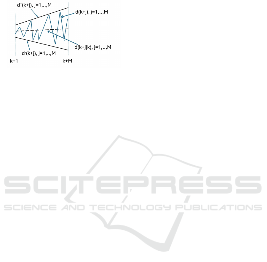
Figure 1: A typical example of volatile customer demand
over P
k
= [k + 1, k + M].
U
k
△
= [u(k|k),··· , u(k + N − 1|k)] be the optimal pre-
dicted sequence of replenishment orders to be com-
puted.
The point-wise bounds u
−
k,i
and u
+
k,i
on u(k + i|k),
i = 0,· ·· ,N − 1, are computed at the beginning of
each H
k
before solving the min-max MPC.
The robust min-max MPC problem is formally de-
fined as follows:
min
U
k
max
ρ∈[ρ
−
,ρ
+
]
J
k
(4)
subject to:(1) − (3) and
u
−
k,i
≤ u(k + i|k) ≤ u
+
k,i
i = 0,·· · , N − 1 (5)
The cost functional J
k
is defined in the following way
J
k
=
N−1
∑
i=0
e
T
(k + L + i|k)q
i
(k)e(k + L + i|k)
+ (∆u(k|k))
T
λ(k)∆u(k|k)
with:
e(k + L + i|k)
△
= (y(k + L + i|k) + u(k + i|k))
− d
+
(k + L + i) (6)
∆u(k|k)
△
= u(k|k) − u(k − 1)
y(k + L + i|k) = ρ
L+i
y(k) +
L−1
∑
ℓ=0
ρ
L+i−ℓ
u(k + ℓ − L)
+
i−1
∑
ℓ=0
ρ
i−ℓ
u(k + ℓ|k)
−ρ
L+i
h(k) −
L+i−1
∑
ℓ=1
ρ
L+i−ℓ
h(k + ℓ|k) (7)
h(k + ℓ|k) = d(k + ℓ|k) + δd(k + ℓ|k) − z(k + ℓ|k)
According to the receding horizon paradigm, over
each H
k
, only the first sample u(k|k) of U
k
is issued
by the retailer to the manufacturer (namely u(k) =
u(k|k)).
Some remarks on J
k
are now in order:
- the tracking error definition (6) is motivated by
R1: the necessity of fulfilling any possible cus-
tomer demand compatible with A5 without incur-
ring overstocking.
- The term ∆u
T
(k|k)λ(k)∆u(k|k) and the hard
constraints (5) have been introduced to satisfy R2:
limiting large deviations on the IRP reduces the
unavoidable costs related to frequent order quan-
tity changes. Forcing the control effort to fluctuate
within a predefined amplitude range allows us to
contain the BE. How to set the limits u
−
k,i
and u
+
k,i
,
i = 0, ··· , N − 1, of this range is explained here
beneath
3.2 The Point-Wise Limits on the
Control Effort
The assumptions on the future customer demand do
not allow computing the hard constraints on the con-
trol effort using the same arguments based on the no-
tion steady-state response used in (Jetto and Orsini,
2024).
Here, the bounds u
−
k,i
and u
+
k,i
, i = 0,··· , N −1 are cal-
culated by an induction process starting from the fol-
lowing assumption:
A6) At a generic time instant k − 1 we have already
determined u
−
k−1,i
and u
+
k−1,i
, i = 0,··· ,N − 1, in such
a way that
e(k − 1 + L + i|k − 1) ≥ 0 i = 0,··· , N − 1, (8)
∀d(k + j) ∈ D
k−1
, j = 1,·· · ,M and ∀ρ ∈ [ρ
−
,ρ
+
]
Remark 1 Note that A6 is a very weak assumption,
because (8) can be trivially satisfied for k = 0 choos-
ing
u
−
0,i
= u
+
0,i
= d
+
(L + i), i = 0,··· ,N − 1 (9)
△
Now, we show that A6 implies that an analogous con-
dition also holds at the next time instant.
Consider the one-step prediction form of (1)
y(k + L + i|k) = ρ [y(k − 1 + L + i|k − 1)
+ u(k − 1 + i|k − 1) − h(k − 1 + L + i|k − 1)] (10)
By (2) and (8), y(k + L + i|k) can be rewritten as:
y(k + L + i|k) = ρ [y(k − 1 + L + i|k − 1)
+ u(k − 1 + i|k − 1) − d(k − 1 + L + i)] (11)
Recalling (6), assumption A6, Remark 1 and (11) it
can be readily seen that
e(k + L + i|k) ≥ u(k + i|k) − d
+
(k + L + i)
+ρ

d
+
(k − 1 + L + i) − d(k − 1 + L + i)

i = 0,·· · , N − 1 (12)
Effective Inventory Control Under Very Large Unknown Deterioration Rate and Volatile, Almost Unpredictable Customer Demand
17

By (12), the minimum u(k + i|k) such that
e(k + L + i|k) ≥ 0 i = 0,··· ,N − 1, (13)
∀d(k + j) ∈ D
k
, j = 1,·· · ,M and ∀ρ ∈ [ρ
−
,ρ
+
]
is
u(k + i|k) = d
+
(k + L + i)
−ρ
−

d
+
(k − 1 + L + i) − d(k − 1 + L + i)

As
d(k −1+L +i) ∈ [d
−
(k −1+L +i),d
+
(k −1+L +i)]
we derive the following limits u
−
k,i
and u
+
k,i
on u(k +
i|k), i = 0, ··· , N − 1
u
−
k,i
= d
+
(k + L + i)
−ρ
−

d
+
(k − 1 + L + i) − d
−
(k − 1 + L + i)

(14)
u
+
k,i
= d
+
(k + L + i) (15)
The amplitude A
k,i
of [u
−
k,i
,u
+
k,i
] is
A
k,i
= ρ
−

d
+
(k − 1 + L + i) − d
−
(k − 1 + L + i)

(16)
Equations (14)-(16) provide an estimate of the BE in
terms of limits on the IRP. Some theoretical consider-
ations on this result are now in order.
Remark 2
• the point-wise upper bound u
+
k,i
coincides with the
maximum admissible value for the current cus-
tomer demand. This prevents an amplification of
u(k + i|k) with respect to any possible maximum
customer demand compatible with A5;
• condition (16) evidences that the amplitude A
k,i
of
[u
−
k,i
,u
+
k,i
] decreases progressively as ρ
−
tends to
0
+
. This is a very positive effect because reduces
the negative impact of large perishability on the
BE (Minner and Transchel, 2017).
We are now in a position to state conditions to obtain
an anti-BE effect, i.e. an IRP taking values inside over
subset of the demand variability range.
Theorem The above point-wise constraints imply
a contraction occurs with respect to the bounds on the
customer demand namely
u(k + i|k) ∈ [u
−
k,i
,u
+
k,i
] ⊂ [d
−
(k + L + i),d
+
(k + L + i)]
(17)
if and only if
∆
k,i
> ρ
−
∆
k−1,i
(18)
where ∆
k,i
△
= d
+
(k + L + i) − d
−
(k + L + i) and
∆
k−1,i
△
= d
+
(k − 1 + L + i) − d
−
(k − 1 + L + i).
Proof By (14),(15), condition (17) holds if and
only if
d
+
(k + L + i) − ρ
−

d
+
(k − 1 + L + i)
−d
−
(k − 1 + L + i)

> d
−
(k + L + i)
namely (18) holds.
4 SOLVING THE MIN-MAX MPC
AS A CONSTRAINED ROBUST
LS PROBLEM
In this section we reformulate the min-max optimiza-
tion problem (4),(5) as a constrained robust LS esti-
mation problem that can be numerically solved much
more efficiently using interior point methods (Lobo
et al., 1998). We define the following vectors:
- u
k
△
= [u(k|k),··· , u(k + N − 1|k)]
T
- ν
l
△
= [0,··· , 0,1,0, ··· , 0] where the element 1 is
in the l-th position (1 ≤ l ≤ N)
- ν
0
is the (1 ×N ) null row vector.
This allows rewriting each element u(k + i|k), i =
0,·· · , N − 1, of the optimal predicted sequence U
k
as
u(k + i|k) = ν
i+1
u
k
(19)
We now show that the column vector u
k
can be com-
puted as the solution of the constrained robust LS es-
timation problem defined beneath.
As ρ ∈ [ρ
−
, ρ
+
], an equivalent representation of ρ is
ρ =
¯
ρ + δρ (20)
where
¯
ρ is the central value of [ρ
−
, ρ
+
] and δρ is the
perturbation with respect to the nominal
¯
ρ . From (20)
it follows that
ρ
ℓ
=
¯
ρ
ℓ
+ ∆ρ
ℓ
(21)
where ∆ρ
ℓ
is the sum of all terms containing the δρ’s,
in the explicit expression of ρ
ℓ
.
Starting from (19) and (21), an equivalent representa-
tion of the predicted tracking error given by (6) is
e(k + L + i|k) = (b
k,i
+ δb
k,i
) − (D
k,i
+ δD
k,i
)u
k
where
b
k,i
△
=
¯
ρ
L+i
y(k) +
L−1
∑
ℓ=0
¯
ρ
L+i−ℓ
u(k + ℓ − L)
−
¯
ρ
L+i
h(k)
−
L+i−1
∑
ℓ=1
¯
ρ
L+i−ℓ
d(k + ℓ|k) − d
+
(k + L + i)
δb
k,i
△
= ∆ρ
L+i
y(k) +
L−1
∑
ℓ=0
∆ρ
L+i−ℓ
u(k + ℓ − L)
− ∆ρ
L+i
h(k) −
L+i−1
∑
ℓ=1
∆ρ
L+i−ℓ
d(k + ℓ|k)
−
L+i−1
∑
ℓ=1
ρ
L+i−ℓ
δd(k + ℓ|k)
+
L+i−1
∑
ℓ=1
ρ
L+i−ℓ
z(k + ℓ|k)
ICORES 2025 - 14th International Conference on Operations Research and Enterprise Systems
18

D
k,i
△
=





−ν
i+1
i = 0
−
h
∑
i−1
ℓ=0
(
¯
ρ
(i−ℓ)
ν
ℓ+1
) + ν
i+1
i
i ≥ 1
δD
k,i
△
=



−ν
i
i = 0
−

∑
i−1
ℓ=0
∆ρ
i−ℓ
ν
ℓ+1

i ≥ 1
Also the term
∆u(k|k) = u(k|k) − u(k − 1)
△
= ν
1
u
k
− u(k − 1)
in J
k
can be rewritten as
∆u(k|k) = (b
u
k
+ δb
u
k
) − (D
u
k
+ δD
u
k
)u
k
where:
b
u
k
= −u(k −1), D
u
k
= −ν
1
, δb
u
k
= 0 and δD
u
k
= ν
0
.
The definition of appropriate extended vectors e
k
, u
−
k
,
u
+
k
, b
k
, δb
k
and matrices D
k
and δD
k
e
k
=






q
1/2
0
(k)e(k + L|k)
.
.
.
q
1/2
N−1
(k)e(k + L + N − 1|k)
λ
1/2
(k)∆u(k|k)






u
−
k
△
=



u
−
k,0
.
.
.
u
−
k,N−1



u
+
k
△
=



u
+
k,0
.
.
.
u
+
k,N−1



(22)
b
k
=






q
1/2
0
(k)b
k,0
.
.
.
q
1/2
N−1
(k)b
k,N−1
λ
1/2
(k)b
u
k






δb
k
=






q
1/2
0
(k)δb
k,0
.
.
.
q
1/2
N−1
(k)δb
k,N−1
λ
1/2
(k)δb
u
k






D
k
=






q
1/2
0
(k)D
k,0
.
.
.
q
1/2
N−1
(k)D
k,N−1
λ
1/2
(k)D
u
k






δD
k
=






q
1/2
0
(k)δD
k,0
.
.
.
q
1/2
N−1
(k)δD
k,N−1
λ
1/2
(k)δD
u
k






allow us to reformulate the min-max MPC (4)-(5) as
the following constrained robust LS estimation prob-
lem:
min
u
k
max
∥δD
k
∥
s
≤β
k
∥δb
k
∥≤ξ
k
∥(b
k
+ δb
k
) − (D
k
+ δD
k
)u
k
∥
2
(23)
subject to u
−
k
≤ u
k
≤ u
+
k
(24)
Exploiting a result of (Lobo et al., 1998), it has been
shown in (Jetto and Orsini, 2024) that at any k, the
solution u
k
of the constrained robust LS estimation
problem (23)-(24) can be determined minimizing the
following sum of euclidean norms
min
u
k
∥b
k
− D
k
u
k
∥ + β
k
∥u
k
∥ + ξ
k
(25)
where u
k
must satisfy (24).
Remark 3 As ξ
k
is independent of u
k
, only the
upper bound β
k
on ∥δD
k
∥
s
in (25) needs to be
determined at each k. The numerical value of β
k
is
determined putting ρ = ρ
+
. △
The theoretical considerations that justify this ap-
proach, mentioned in the Introduction, are reported
in the following remark.
Remark 4 Feasibility of constraints (5) derives
from: (19) and the consistency of (24) w.r.t. (23).
The internal asymptotic stability of the controlled
SC derives from: i) 0 < ρ < 1, ii) d(k) ≤
¯
d < ∞,
k ∈ Z
+
, iii) constraints (5). As the stated properties of
stability and feasibility are independent of the length
of the prediction horizon, it follows that assumption
A5 can be limited to very short intervals P
k
, only
depending on the actual knowledge about the limits
on the future customer demand.
5 NUMERICAL SIMULATIONS
We consider a highly perishable single echelon SC
whose dynamics equation (1) is characterized by a
lead time L = 1 and a very large uncertain DF α ∈
[α
−
,α
+
] = [0.45, 0.5] or, equivalently an uncertain
decay factor ρ ∈ [ρ
−
,ρ
+
] = [0.5,0.55].
According to A5, at each k ∈ Z
+
and over a very short
M-steps prediction interval P
k
with M = 2, the un-
known future demand is arbitrarily varying inside a
given compact set D
k
. The profile of the whole, as-
sumed, actual customer demand d(k) is the irregular
continuous line shown in Fig. 2. The dashed lines are
the boundaries of the compact set D enclosing d(k).
The dynamic equation (1) of the actual SC is imple-
mented assuming an actual decay factor ρ = 0.53.
The parameters defining the min max MPC al-
gorithm are the length N = 2 = M − L + 1 of H
k
(control horizon) and the weights of (6): q
i
(k) =
1
(0.01·d
+
(k+L+i))
2
e
−i
, λ(k) =
1
(0.01·u(k−1))
2
for k ≥ 1,
λ(0) = 1 chosen according to the guidelines given in
(G.F. Franklin, 1990). The simulation is stopped at
time k = 40. The ordering signal u(k) obtained is re-
ported in Fig. 3. This figure clearly shows the limi-
tation of the BE: u(k) has a smoother waveform than
the customer demand and is contained in a narrower
range. The actual (d(k)) and fulfilled (h(k)) customer
demands are shown in Fig. 4. The almost total over-
lap of the two curves evidences the effectiveness of
the proposed method: the percentage of Unsatisfied
Customer Demand defined as
UCD =
∑
40
k=0
|d(k) − h(k)|
∑
40
k=0
d(k)
× 100 (26)
Effective Inventory Control Under Very Large Unknown Deterioration Rate and Volatile, Almost Unpredictable Customer Demand
19

0 5 10 15 20 25 30 35 40
k review period
0
20
40
60
80
100
120
140
the customer demand d(k) (solid line)
Figure 2: The actual customer demand d(k) (solid line). The
dashed lines delimit the compact set D given by the consec-
utive contiguous overlapping of all the ”a priori” given sets
D
k
’s.
0 5 10 15 20 25 30 35 40
k review period
0
20
40
60
80
100
120
140
the generated order signal u(k) (solid line)
Figure 3: The generated ordering signal u(k) (solid line)
and the boundaries trajectories (dashed lines) computed by
(14)-(15).
0 5 10 15 20 25 30 35 40
k review period
0
20
40
60
80
100
120
140
d(k) (solid line), h(k) (dashed line)
Figure 4: The customer demand d(k) (solid line) and the
fulfilled customer demand h(k) (dashed line). The two tra-
jectories are overlapped for k ≥ L.
results to be UCD = 1.1%.
0 5 10 15 20 25 30 35 40
k
review period
0
50
100
150
200
250
300
The generated order signal u(k) (solid line)
Figure 5: (OUT policy) The generated ordering signal u(k)
(solid line).
5.1 Comparison with the Order up to
(OUT) Policy
With reference to the same SC, we compare our
method with an OUT policy. To take into account the
presence of perishable goods, of a time delay and of
an uncertain future customer demand, we propose a
version of the OUT policy where the predicted inven-
tory level y(k + L + 1|k) coincides with the possible
maximum value of the demand d
+
(k + L + 1) in ac-
cordance with A5. The replenishment policy is com-
puted solving (7) with respect to the single sample
u(k|k)
△
= u(k) setting i = 1. To guarantee customer
satisfaction according to a precautionary worst case
approach we also assume:
- y(k + L + 1|k) = d
+
(k + L + 1);
- h(k + ℓ|k) = d(k + ℓ) = d
+
(k + ℓ), ℓ = 1,·· · ,L,
- ρ = ρ
−
Solving (7) gives
u(k) =
1
ρ
−

d
+
(k + L + 1) + (ρ
−
)
L+1
h(k)
+
L
∑
ℓ=1
(ρ
−
)
L+1−ℓ
d
+
(k + ℓ) − (ρ
−
)
L+1
y(k)
−
L−1
∑
ℓ=0
(ρ
−
)
L+1−ℓ
u(k + ℓ − L)
!
(27)
With the same fulfilled demand (the UCD perfor-
mance index is the same) the OUT policy yields a
higher replenishment order (compare figure 3 with 5)
leading to performance degradation in terms of BE
containment and excessive inventory.
6 CONCLUSIONS
Suitably exploiting the flexibility and generality of
min-max MPC we defined an optimal and robust IRP
ICORES 2025 - 14th International Conference on Operations Research and Enterprise Systems
20

to effectively counteract the negative effects of the as-
sumed very critical operating conditions. In this con-
text, the result on the point-wise hard constraints rep-
resents a more general key theoretical contribution to-
wards the solution of the very long-standing problem
of controlling the BE. Numerical simulations show
the effectiveness of the method in reconciling the two
opposing requirements R1 and R2.
7 FUTURE WORK
Possible and promising developments of this ap-
proach concern the extension to the case of an uncer-
tain time varying decay factor.
REFERENCES
Abolghasemia, M., Beha, E., Tarrb, G., and Gerlachc, R.
(2020). Demand forecasting in supply chain: The im-
pact of demand volatility in the presence of promo-
tion. Computers & Industrial Engineering, 142.
Carlson, J. and Doyle, J. (2002). Complexity and robust-
ness. In Proceedings of the National Academy of Sci-
ences. PubMed.
Chaudary, V., Kulshrestha, R., and Routroy, S. (2018). State
of the art literature review on inventory models for
perishable products. Journal of Advances in Manage-
ment Research, 1:306–346.
De-Boor, C. (1978). A practical guide to splines. Springer
Verlag, New York, 2nd edition.
Gaggero, M. and Tonelli, F. (2015). Optimal control of dis-
tribution chains for perishable goods. IFAC Papers On
Line, 48:1049–1054.
G.F. Franklin, J.D. Powell, M. W. (1990). Digital Control of
Dynamic Systems. Addison-Wesley Publishing Com-
pany, N.Y, 2nd edition.
Hipolito, T., Nabais, J., Benitez, R., Botto, M., and Negen-
born, R. (2022). A centralised model predictive con-
trol framework for logistics management of coordi-
nated supply chain of perishable goods. International
Journal of Systems Science: Operation & Logistics,
9:1–21.
Ietto, B. and Orsini, V. (2022a). Effective inventory control
in supply chain with large uncertain decay factor. In
30th Mediterranean Conference on Control and Au-
tomation. IEEE.
Ietto, B. and Orsini, V. (2022b). Resilient robust model
predictive control of inventory systems for perish-
able good under uncertain forecast information. In
2022 International Conference on Cyber-physical So-
cial Intelligence (Best paper finalists award). IEEE.
Ietto, B. and Orsini, V. (2023a). Managing inventory level
and bullwhip effect in multi stage supply chains with
perishable goods: A new distributed model predic-
tive control approach. In 12th International Confer-
ence on Operations Research and Enterprise Systems.
SCITEPRESS.
Ietto, B. and Orsini, V. (2023b). Optimal control of inven-
tory level for perishable goods with uncertain decay
factor and uncertain forecast information: a new ro-
bust mpc approach. International Journal of Systems
Science: Operations & Logistics, 10:1–13.
Ietto, B. and Orsini, V. (2024). The notion of internal
dynamics and its impact on modeling and control-
ling supply chains with goods characterized by uncer-
tain perishability rate. IEEE Transactions on Systems,
Man, and Cybernetics: Systems, 54:7356–7368.
Jetto, B. and Orsini, V. (2024). Resilient and robust manage-
ment policy for multistage supply chains with perish-
able goods and inaccurate forecast information: A dis-
tributed model predictive control approach. Optimal
Control: Applications and Methods, 45:2383–2414.
Lejarza, F. and Baldea, M. (2020a). Closed-loop optimal
operational planning of supply chains with fast prod-
uct quality dynamics. Computers and Chemical Engi-
neering, 132:1–16.
Lejarza, F. and Baldea, M. (2020b). Closed-loop real-
time supply chain management for perishable prod-
ucts. IFAC PapersOnLine, 53:11458–14463.
Lobo, M., Vandenberghe, L., Boyd, S., and L
´
ebret, H.
(1998). Second-order cone programming. Linear Al-
gebra and its Applications, 284:193–218.
Minner, S. and Transchel, S. (2017). Order variability in
perishable product supply chains. European Journal
of Operational Research, 260:93–107.
Rossiter, J. and Bishop, R. (2004). Model Based Predictive
Control. A Practical Approach. CRC PRESS, Boca
Raton, 1st edition.
Taparia, R., Janardhanan, S., and Gupta, R. (2020). Inven-
tory control for nonperishable and perishable goods
based on model predictive control. International
Journal of Systems Science: Operations & Logistics,
7:361–373.
Effective Inventory Control Under Very Large Unknown Deterioration Rate and Volatile, Almost Unpredictable Customer Demand
21