On the Prediction of a Nonstationary Geometric Distribution
Based on Bayes Decision Theory
Daiki Koizumi
a
Otaru University of Commerce, 3–5–21, Midori, Otaru-city, Hokkaido, 045–8501, Japan
Keywords:
Probability Model, Bayes Decision Theory, Nonstationary Geometric Distribution, Hierarchical Bayesian
Model, Time Series Analysis.
Abstract:
This paper considers a prediction problem with a nonstationary geometric distribution in terms of Bayes de-
cision theory. The proposed nonstationary statistical model contains a single hyperparameter, which is used
to express the nonstationarity of the parameter of the geometric distribution. Furthermore, the proposed pre-
dictive algorithm is based on both the posterior distribution of the nonstationary parameter and the predictive
distribution for data, operating with a Bayesian context. Each predictive estimator satisfies the Bayes optimal-
ity, which guarantees a minimum mean error rate with the proposed nonstationary probability model, a loss
function, and a prior distribution of the parameter in terms of Bayes decision theory. Furthermore, an approxi-
mate maximum l ikelihood estimation method for the hyperparameter based on numerical calculation has been
considered. Finally, the predictive performance of the proposed algorithm has been evaluated in terms of both
the model selection theory and the predictive mean squared error by comparison with the stationary geometric
distribution using real web tr affic data.
1 INTRODUCTION
The geometric distribution (Johnson and Kotz, 1969)
(Hogg et a l., 2013) is one of significan t discr e te prob-
ability distributions with at least two defin itions. One
is that the probability distribution of the number of
failures before the first success, with the suc cess prob-
ability as the parameter. The other is th at the discrete
probability distribution of the number of Bernoulli tri-
als needed to get one success given the same param-
eter. This paper is based on the former definition.
Some important characteristics of the g e ometric dis-
tribution ar e that it is the discrete version of the expo-
nential distribution; that it has the memoryless prop-
erty; and that it is a special case of the negative bino-
mial distribution. Based on the above definitions and
characteristics of the geometr ic distribution, many ap-
plications have been reported, including quality con -
trol ( Frank C. Kaminsky and Burke, 1992), queu e ing
theory (Winsten , 1959 ), biology (Ewe ns, 2004), ep i-
demiology (O. Diekmann, 2000), co mmunication the-
ory (G.G allager, 1995), computer networks (Bianchi,
2000), and so forth.
a
https://orcid.org/0000-0002-5302-5346
In the field of Bayesian statistics (Berger, 1985)
(Bernardo and Smith, 1994), on th e o ther hand, the
parameter estimation or prediction problems often be-
come intracta ble. This is because these problems re-
quire integral calculation s in the denominator of the
Bayes theorem depending on a known prior distribu-
tion o f parameter. However, if the specific distribu-
tion of parameter is assumed to be the prior, com-
plex integral calculations can be avoided. In Bayesian
statistics, th is specific class of prior is called a con-
jugate family (Berger, 1985, pp. 130–132 ) (Bernardo
and Smith, 1994, pp. 265–267). The beta distribution
is the natural conjugate prior of the stationary geomet-
ric distribution (Bernardo and Smith, 1994).
The above results are limited within th e stationary
geometric distribution. If the nonstationary probabil-
ity distributions are assumed, the Bayesian estimation
problems become more difficult and more intractable .
In such cases, there is no gua rantee of the existence
of a natural conjugate prior. In this regard, at least
two nonstationary probability m odels h ave been pro-
posed. One is the Bayesian entropy forecasting (BEF)
model (Souza, 1978) in which the Sha nnon’s entropy
function and Jaynes’ principle of maximum entropy
are applied to the model formulation. The other is re-
ferred to as the Simp le Power Steady Model (SPSM)
140
Koizumi, D.
On the Prediction of a Nonstationary Geometric Distribution Based on Bayes Decision Theory.
DOI: 10.5220/0013097500003890
Paper published under CC license (CC BY-NC-ND 4.0)
In Proceedings of the 17th International Conference on Agents and Artificial Intelligence (ICAART 2025) - Volume 3, pages 140-149
ISBN: 978-989-758-737-5; ISSN: 2184-433X
Proceedings Copyright © 2025 by SCITEPRESS – Science and Technology Publications, Lda.

(Smith, 1979). The SPSM is a time-series model and
they have shown certain illustrative probability distri-
butions called linear expanding families in w hich nat-
ural conjugate priors exist (Smith, 1979). Recently,
a new similar and particular nonstationary parame-
ter cla sses with hy perparameter estimation methods
have been proposed (Koizumi, 2020; Koizumi, 202 1;
Koizumi, 2023). Among the aforementioned results,
a single hyperparameter is identified as the expression
of n onstationarity of the parameter, and its estima -
tion can be achieved through the approximate max-
imum likelihood estimatio n with nu merical calcula-
tion. T hese results contribute new aspects to the field
of empirical Bayes methods (Carlin and Louis, 2000).
Furthermore, a Bayesian problem in the context of
Bayes decision theory (Berger, 1985) (Bernardo and
Smith, 1994) has be e n c onsidered. Using this ap -
proach , the predictive estimator satisfies Bayes opti-
mality, which guar a ntees a minimum m e an error rate
for predictio ns.
In this paper, the aforementioned app roach to
the n onstationary geometric d istribution is presented.
The pr oposed nonstation ary class of parameter has
only a single hyperparameter. This hyperpara meter
can be estimated from obser ved data by an approx-
imate maximum likelihood estimation with numer-
ical calculations. Under condition with the known
(or estimated) hyper parameter, the posterior distribu-
tion of parameter with specific prior can be tracta bly
obtained with simpler arithmetic calculations. This
point would b e the generalization of the natural con-
jugate prior with stationary geometric distribution to
avoid heavy integral calculations under the equation
of Bayes theorem. Moreover, a Bayes optimal pre-
diction algorithm is proposed, which guarantees the
a minimum me an err or rate for p redictions in terms
of Bayes decision theory. Finally, evaluation of the
predictive performances of the proposed algorithms
are via comparison with the results of the stationary
geometric distribution using real web traffic data is
detailed.
The rest of this paper is organized as follows. Sec-
tion 2 provides th e basic definitions of the prop osed
nonstationary geometric distribution and some lem-
mas a nd corollaries in terms of Bayesian statistics.
Section 3 proposes the Bayes optimal predictive al-
gorithm in terms of Bayes decision theory. Section
4 presents numeric al exam ples using real web traffic
data. Section 5 presents a discussion on the results of
this paper. Section 6 presents the conclusion.
2 PRELIMINARIES
2.1 Hierarchical Bayesian Modeling
with Nonstatio nary Geometric
Distribution
Let t = 1, 2, .. . be a discrete time index and X
t
= x
t
≥
0 be a discrete random variable at t. Assume that
x
t
= 0, 1, 2, . . . , N represents co unt data with known
N and X
t
∼ Geo metric (θ
t
), where 0 < θ
t
≤ 1, is a
nonstationary parameter at t. Thus, the probability
function of the nonstationary geometric distribution
p

x
t


θ
t

is defined as follows:
Definition 2.1. Nonstationary Geometric Distribu-
tion
p

x
t


θ
t

= (1 − θ
t
)
x
t
θ
t
, (1)
where x
t
= 0, 1, 2, . . . , N and 0 < θ
t
≤ 1. ✷
Definition 2.2. Fun ction fo r Θ
t
, A
t
, and B
t
Let Θ
t
= θ
t
, A
t
= a
t
, and B
t
= b
t
be random vari-
ables where A
t
and B
t
are mutually independent, the n
a function for Θ
t
is defined as,
Θ
t
=
A
t
A
t
+ B
t
, (2)
where 0 < a
t
, 0 < b
t
. ✷
Definition 2.3. Nonstationarity of A
t
, B
t
Let C
t
= c
t
, D
t
= d
t
be random variables, th en the non-
stationary function s for A
t
and B
t
are defined as,
A
t+1
= C
t
A
t
, (3)
B
t+1
= D
t
B
t
, (4)
where 0 < c
t
< 1, 0 < d
t
< 1 and they are sampled
from the following two type s of beta distributions:
C
t
∼ Beta [kα
t
, (1 − k)α
t
] , (5)
D
t
∼ Beta [kβ
t
, (1 − k)β
t
] , (6)
where k is a real valued constant and 0 < k ≤ 1 . ✷
Definition 2.4. Conditional In dependence for A
t
,C
t
(or B
t
, D
t
) under α
t
(or β
t
)
p

a
t
, c
t


α
t

= p

a
t


α
t

p

c
t


α
t

, (7)
p

b
t
, d
t


β
t

= p

b
t


β
t

p

d
t


β
t

. (8)
✷
Definition 2.5. In itial Distributions for A
1
, B
1
A
1
∼ Gamma (α
1
, 1) , (9)
B
1
∼ Gamma (β
1
, 1) , (10)
where 0 < α
1
and 0 < β
1
. ✷
On the Prediction of a Nonstationary Geometric Distribution Based on Bayes Decision Theory
141

Definition 2.6. Initial Distributions for C
1
, D
1
C
1
∼ Beta [kα
1
, (1 − k)α
1
] , (11)
D
1
∼ Beta [kβ
1
, (1 − k)β
1
] . (12)
✷
Definition 2.7. Gamma Distribution for q
Gamma distribution of Gamma (r, s) is defined as,
p

q


r, s

=
s
r
Γ(r)
q
r−1
exp(−sq) , (13)
where 0 < q, 0 < r, 0 < s, an d Γ(r) is the gamma func-
tion defined in Definition 2.9. ✷
Definition 2.8. Beta Distribution for q
Beta distribution of Beta (r, s) is defined as,
p

q


r, s

=
Γ(r + s)
Γ(r) Γ(s)
q
r−1
(1 − q)
s−1
, (14)
where 0 < q < 1, 0 < r, 0 < s. ✷
Definition 2.9. Gamma Func tion for q
Γ(q) =
Z
+∞
0
y
q−1
exp(−y)dy , (15)
where 0 < q . ✷
2.2 Lemmas
Lemma 2.1. Transformed Distribution for A
t
For any t ≥ 1, the transformed random variable
A
t+1
= C
t
A
t
in Definition 2.3 follows the following
Gamma distribution:
A
t+1
∼ Gamma (kα
t
, 1) . (16)
✷
Proof of Lemma 2.1.
See APPENDIX A. ✷
Lemma 2.2. Transformed Distribution for B
t
For any t ≥ 1, the transformed rando m variable
B
t+1
= D
t
B
t
in Definition 2.3 follows the following
Gamma distribution:
B
t+1
∼ Gamma (kβ
t
, 1) . (17)
✷
Proof of Lemma 2.2.
The proof is exactly same as Lemma 2 .1, replacing
A
t+1
by B
t+1
, C
t
by D
t
, and α
t
by β
t
.
This complete s the proof of Lemma 2 .2. ✷
Lemma 2.3. Transformed Distribution for Θ
t
For any t ≥ 2, the transfor med random variable Θ
t
=
A
t
A
t
+B
t
in Definition 2.2 follows the following beta dis-
tribution:
Θ
t
∼ Beta (kα
t−1
, kβ
t−1
) . (18)
✷
Proof of Lemma 2.3.
See APPENDIX B. ✷
Corollary 2 .1. Transformed Initial Distribution for
Θ
1
The transformed random variable Θ
1
=
A
1
A
1
+B
1
in
Definition 2.2 follows the following beta distribution:
Θ
1
∼ Beta (α
1
, β
1
) . (19)
✷
Proof of Corollary 2.1.
From Definition 2.5,
A
1
∼ Gamma (α
1
, 1) ,
B
1
∼ Gamma (β
1
, 1) .
If Lemma 2.3 is applied to the above A
1
and B
1
, then
the following holds,
Θ
1
∼ Beta (α
1
, β
1
) . (20)
This completes the proof of Corollary 2.1. ✷
3 PREDICTION ALGORITHM
BASED ON BAYES DECISION
THEORY
3.1 Preliminaries
Definition 3.1. Loss Function
In this paper, the predictive error for x
t+1
is measured
by the following squared-error loss function (Berger,
1985, 2.4.2, I., p. 60),
L( ˆx
t+1
, x
t+1
) = ( ˆx
t+1
− x
t+1
)
2
. (21)
✷
Definition 3.2. Risk Function
The risk function is defined as the expectation of the
loss function L( ˆx
t+1
, x
t+1
) with respect to the sam-
pling distribution p

x
t+1


θ
t+1

,
R ( ˆx
t+1
, θ
t+1
)=
N
∑
x
t+1
=0
L( ˆx
t+1
, x
t+1
)p

x
t+1


θ
t+1

,(22)
where p

x
t+1


θ
t+1

is from Definition 2.1. ✷
Definition 3.3. Bayes Risk Fun c tion
Let x
x
x
t
= (x
1
, x
2
, . . . , x
t
) be observed sequence and
p

θ
t


x
x
x
t

be th e posterior distribution of pa rameter θ
t
under x
x
x
t
. Then, the posterior distribution after param-
eter transitions to nonstationary becomes p

θ
t+1


x
x
x
t

and the Bayes Risk Func tion BR ( ˆx
t+1
) is defined as,
BR (ˆx
t+1
)=
Z
1
0
R ( ˆx
t+1
, θ
t+1
) p

θ
t+1


x
x
x
t

dθ
t+1
. (23)
✷
ICAART 2025 - 17th International Conference on Agents and Artificial Intelligence
142

Definition 3.4. Bayes Optimal Prediction
The Bayes optimal prediction ˆx
∗
t+1
is defined as the
minimizer of the Baye s r isk fu nction,
ˆx
∗
t+1
= argmin
ˆx
t+1
BR (ˆx
t+1
) . (24)
✷
3.2 Main Theorems
Theorem 3.1. Posterior Distribution after transitions
to nonstationary for θ
t
Let the prior distribution of pa rameter θ
1
of
the nonstationary geometric distribution in Defini-
tion 2.1 be Θ
1
∼ Beta (α
1
, β
1
). For any t ≥ 2,
let x
x
x
t−1
= (x
1
, x
2
, . . . , x
t−1
) be the observed data se-
quence. Then , the posterior distribution of Θ
t


x
x
x
t−1
can be obtained as the following closed form:
Θ
t


x
x
x
t−1
∼ Beta (α
t
, β
t
) , (25)
where the parameters α
t
, β
t
are given as,







α
t
= k
t−1
α
1
+
t−1
∑
i=1
k
i
;
β
t
= k
t−1
β
1
+
t−1
∑
i=1
k
i
x
t−i
.
(26)
✷
Proof of Theorem3.1.
For any t ≥ 2, the posterior of parameter distribu-
tion p

θ
t


x
x
x
t−1

remains in the closed form Θ
t
∼
Beta (α
t
, β
t
) if X
t
∼ Geometric (θ
t
) in De finition 2.1
and Θ
1
∼ Beta (α
1
, β
1
) in Co rollary 2.1 according to
the nature of conjugate families (Bernardo and Smith,
1994, 5.2, p.265) (Berger, 1985, 4.2.2, p.130).
Furthermore, assuming that x
t−1
is the observed
data,

α
t
= α
t−1
+ 1;
β
t
= β
t−1
+ x
t−1
,
(27)
holds for t ≥ 2 by conjugate a nalysis (Bernardo and
Smith, 1994, n = 1, r = 1 for Negative-Binomia l
model, p.43 7). This is the proof of Eq. (25).
In this paper, nonstationary parameter model is as-
sumed. Therefore, if both Lemma 2.1, and Lemma
2.2 are recursively applied to Eq. (27), then,

α
t
= k (α
t−1
+ 1);
β
t
= k (β
t−1
+ x
t−1
) ,
(28)
holds for t ≥ 2.
Finally, Eq. (26) is ultimately derived by recur-
sively applying Eq. (28) backwards until the initial
conditions α
1
, β
1
in both Definition 2.5 and Corollary
2.1 are reached.
This complete s the proof of Theorem 3.1. ✷
Remark 3.1.
The right hand sid e s of Eq s. (26) have structures
called as Exponentially Weighted Moving Average
(EWMA) (Harvey, 1989). ✷
Theorem 3.2. Predictive Distribution for x
t+1
p(x
t+1


x
x
x
t
) =
α
t+1
∏
x
t+1
−1
i=0
(β
t+1
+ i)
∏
x
t+1
i=0
(α
t+1
+ β
t+1
+ i)
, (29)
where α
t+1
and β
t+1
are formulated in Eq. (26). ✷
Proof of Theorem 3.2 .
p

x
t+1


x
x
x
t

=
Z
1
0
p

x
t+1


θ
t+1

p

θ
t+1


x
x
x
t

dθ
t+1
(30)
=
Γ(α
t+1
+β
t+1
)
Γ(α
t+1
)Γ(β
t+1
)
Γ(α
t+1
+1)Γ(β
t+1
+ x
t+1
)
Γ(α
t+1
+1+β
t+1
+ x
t+1
)
(31)
=
α
t+1
∏
x
t+1
−1
i=0
(β
t+1
+ i)
∏
x
t+1
i=0
(α
t+1
+ β
t+1
+ i)
. (32)
Note that the second term in Eq. (31 ) is obtained fr om
the definition of the beta function and that Eq . ( 32)
is obtained from Eq. (31) by applying the following
property of gamma function: Γ(x + 1) = xΓ(x).
This completes the proof of Theorem 3 .2. ✷
Theorem 3.3. Bayes Optimal Prediction ˆx
∗
t+1
ˆx
∗
t+1
=
β
t+1
α
t+1
− 1
, (33)
where α
t+1
and β
t+1
are formulated in Eq. (26). ✷
Proof of Theorem 3.3 .
For parameter estimatio n problem under the squared -
error loss function, the posterior mean is the optimal
(Berger, 1985, Result 3 and E xample 1, p. 161). For
the prediction prob le m, the p redictive mean, i.e. the
expectation of the Bayes predictive distribution is
identically the optimal under the squared-error loss
function. Therefore,
ˆx
∗
t+1
= E

x
t+1


x
x
x
t

(34)
=
N
∑
x
t+1
=0

x
t+1
p

x
t+1


x
x
x
t

(35)
=
β
t+1
α
t+1
− 1
. (36)
Note that Eq. (36) is derived from Eq. ( 35) by the
expectation of the Negative-Binomial-Beta distribu-
tion (Bernardo and Smith, 1994, p. 42 9).
This completes the proof of Theorem 3 .3. ✷
On the Prediction of a Nonstationary Geometric Distribution Based on Bayes Decision Theory
143

3.3 Hyperparameter Estimation with
Empirical Bayes Method
Since a hyp erparameter 0 < k ≤ 1 in Eqs. (5) and (6)
is assumed to be known, it must be estimated in prac-
tice. In this paper, the following ma ximum likelihood
estimation in terms of empirical Bayes method (Car-
lin and Louis, 2000) is co nsidered.
Let l(k) be a likelihood function of hyperparam-
eter k and
ˆ
k be the maximum likelihood estimator.
Then, those two functions are d efined as,
ˆ
k = argmax
k
l(k), (37)
l(k) = p(x
1


θ
1
)p(θ
1
)
t
∏
i=2
p(x
i


x
x
x
i−1
, k) (38)
=
t
∏
i=1
"
α
i
∏
x
i
−1
j=0
(β
i
+ j)
∏
x
i
j=0
(α
i
+ β
i
+ j)
#
, (39)
where α
i
and β
i
are formulated in Eq. (26).
Eq. (39) can not be solved analytically and then
the approximate numerical calculation meth od should
be applied. The detail is described in Subsection 4.3.
3.4 Proposed Predictive Algorithm
The proposed predictive algorithm that calculates the
Bayes optimal prediction ˆx
∗
t+1
in Theorem 3.3 is de-
scribed as the following Algorithm 3.1.
Algorithm 3.1. Proposed Predictive Algorithm.
1. Estimate hyperparame te r
ˆ
k by Eq. (39) fro m train-
ing data.
2. De fine hyperparam eters α
1
, β
1
for the initial prior
p(θ
1


α
1
, β
1
) in Eqs. (9) and (10).
3. Using the observed sequence x
x
x
t
of test data, cal-
culate the Bayes optimal prediction ˆx
∗
t+1
from
Eq. (33) where α
t+1
and β
t+1
are formulated in
Eq. (26), and k is replaced by
ˆ
k in step 1. in
Eq. (26).
✷
4 NUMERICAL EXAMPLES
4.1 Data Specifications
In order to evaluate the efficacy of the proposed Al-
gorithm 3.1, the real web traffic data is utilized . This
data is extrac te d from the http (Hyper Text Transfer
Protocol) request arrival time stamps at three-minute
intervals from a web server, spanning a twelve-day
period between Ma rch 20 and March 31, 2005.
Tables 1 and 2 illustrate a portion of the speci-
fications of both train ing and test data. Table 1 ex-
plains an overview of the training data on March 25,
2005,while Table 2 provides an overview of the test
data o n March 26, 2005. Figure 1 depicts both plots
with line graphs. In figure 1, the vertical axis rep-
resents the number of r equest ar rivals, the horizontal
axis represents the time in terval index, the blue line
represents the training data, and the red line repre-
sents the te st data.
The remaining characteristics of the data are illus-
trated in Tables 7 and 8 in Appendix C.
Table 1: Training Data Specifications.
Items Values
Date Mar. 25, 2005
Time Interval Every 3 minu te s
Tota l Request Arrivals 11, 527
Tota l Time Intervals t
max
305
Auto Correlation
Coefficient (lag=1 ) 0.821
Table 2: Test Data Specifications.
Items Values
Date Mar. 26, 2005
Time Interval Every 3 minu te s
Tota l Request Arrivals 6, 369
Tota l Time Intervals t
max
291
Auto Correlation
Coefficient (lag=1 ) 0.670
0
20
40
60
80
100
120
140
0 50 100 150 200 250 300
Numbers of Request Arrivals
Time Interval Index
Training Data
Test Data
Figure 1: Training and Test Dat a Plots for Web Traffic Data
on Mar. 25–26, 2005.
4.2 Conditions and Criteria for
Evaluation
The perf ormance of Algorithm 3.1 with the real data
is evaluated. Note that the training data is used only
for hy perparameter estimation of
ˆ
k in Eq. (39). With
the estimated
ˆ
k, the Bayes optimal prediction of ˆx
∗
t+1
ICAART 2025 - 17th International Conference on Agents and Artificial Intelligence
144

is calculated from the test data. For the comparison,
two types of prediction ˆx
∗
t
are considered. The first is
from the proposed algorithm with nonstationary ge-
ometric distribution in Theo rem 3.3 and the second
is from a conventional algorithm with stationary geo-
metric distribution.
4.2.1 Initial Prior Distribution of Parameter
According to Corollary 2.1, the class of th e initial
prior distribution of parame ter is beta distribution.
If the non-informative prior (Berger, 1985; Bernardo
and Smith, 1994) is considered un der beta prior p(θ
1


α
1
, β
1
), it should correspond to the uniform distribu-
tion and each of two hype rparameters of α
1
and β
1
equals to one. Their settings are shown in Table 3.
Table 3: Defined Hyperparameters for Prior Distribution
p

θ
1


α
1
, β
1

.
Items α
1
β
1
Valu es 1 1
4.2.2 Criteria
For the criteria for evaluations, the following mean
squared error ba sed on the squared-error loss function
in Definition 3.1 is defined.
Definition 4.1. Mean Squared Error
1
t
max
t
max
∑
t=1
L( ˆx
t
, x
t
) =
1
t
max
t
max
∑
t=1
( ˆx
t
− x
t
)
2
. (40)
4.3 Results
Table 4 presents the estimated hyperp arameter
ˆ
k from
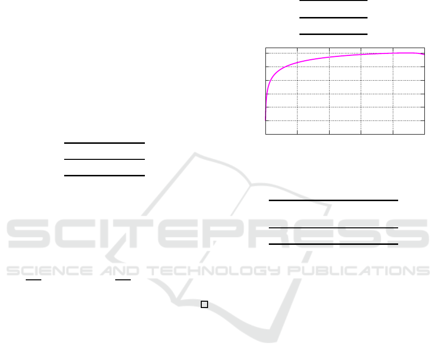
the training data. Figure 2 depicts the loglikelihood
function log l(k) with base of 10
3
, as calculated nu-
merically using R version 4.4.1 (R Core Team, 2024).
Table 9 in Appendix C illustrates the extended re-
sults of th e hyperparameter estimation of the training
data.
Table 5 illustrates the values of predictive mean
squared errors for both the proposed and stationary
models in Definition 4.1. Figure 3 depicts its graphi-
cal r esult. In Figure 3, the h orizontal and vertical axes
are the index of time interval 1 ≤ t ≤ 291 and the num-
ber of request arrivals, respectively. Furthermore, the
orange bar is real request arrivals x
t
from test data, the
blue solid line is the predictions ˆx
∗
t
from the proposed
nonstationary geom etric model, the red solid line is
the predictions from the stationary geometric model.
The second column from Left in Table 10 in Ap-
pendix C illu stra te s the extended results of mean
squared errors for both the proposed and stationary
models from the test data.
Table 4: Hyperparameter Estimation from Training Data.
Item
ˆ
k
Valu e 0.889
-500
-450
-400
-350
-300
-250
-200
0 0.2 0.4 0.6 0.8 1
Loglikelihood
k
Figure 2: log l(k) Plot for 0 ≤ k ≤ 1.
Table 5: Mean Squared Error for Two Models.
Items MSE
Proposed Stationary
Valu es 18 6.8 254.1
5 DISCUSSIONS
From Table 4, the estimator is
ˆ
k = 0.889. If k = 1,
then the second parameter s of beta distributions in
Eqs. (5),(6),(11), and (12) become zero. This means
that the variances of beta distributions a re also zero,
and that the parameter θ
t
of geometric d istribution is
stationary. Therefore
ˆ
k = 0.88 9 6= 1.0 00 m e ans that
training data is nonstationary. Furthermore , Figure 2
show that the likelihood functio n l(k) is empirically
upward convex. Hence the estimated value for
ˆ
k can
be considered reliable as an estimato r.
Table 5 shows that the performance of predic-
tion with th e proposed model is superior to that of
the statio nary model. The improvement of MSE is
more than 25%. In fact, Figure 3 also shows that
the blue line follows the orange bar better than the
red line. Similarly, Figure 4 compares the expecta-
tion values of the p osterior parameter distributions
E

θ
t


x
x
x
t−1

between two models. In Fig ure 4, the
blue line of the proposed model shows more intense
dynamic fluctuations than the red line of the station-
ary model. These results suggest th a t the proposed
empirical Bayesian method with the nonstationary ge-
On the Prediction of a Nonstationary Geometric Distribution Based on Bayes Decision Theory
145

0
20
40
60
80
100
120
0 50 100 150 200 250
Numbers of Request Arrivals
Time Interval Index
Observed Values
Proposed
Stationary
Figure 3: Prediction Result for Test Data.
ometric model works to some extent compared to the
stationary model. However, Figure 3 also shows that
the blue line did not necessarily follow the rapid in-
crease or decrease in th e orange bars. If one sets the
hyperparameter k = 0.50, then the nonstationarity of
parameter θ
t
becomes larger an d the MSE of the pro-
posed model becomes 148.5. In this case, the im-
provement is about 40% better than that of the sta-
tionary mod e l. This desirable situation did not occur
because the training and test data were very different
as shown in Figure 1.
Finally, the values of A kaike Infor mation Criteria
(AIC) (Akaike, 1973) between two models in terms
of the model selection were calculated and shown in
Table 6. Note that the value of AIC is calculated by
(−2 log
2
L + 2m), where L and m represent the likeli-
hood value and the number of parameters in the statis-
tical model, respectively. In this paper, m = 4 for the
proposed nonstationary model (θ
t
, α
t
, β
t
, and k) and
m = 3 for the stationary model (θ
t
, α
t
, and β
t
). There-
fore, the parametric penalty in AIC for the proposed
model did not become so larger th a n that of the sta-
tionary model. As a result, the value of AIC in Table
6 for the proposed model is sligh tly smaller than that
of the stationary model. It means that the proposed
model is relatively suitable than the stationary model.
Furthermore, the third and fourth columns of Table
9 in Appendix C presen t the extended results of the
AIC values for the training data. The overall results
indicate that the the proposed nonstationar y geomet-
ric model is compa ratively mor e suitable than the sta-
tionary geometric model based on the observed data
in terms of the model selectio n.
Table 6: A kaike Information Criteria (A I C) for Two Mod-
els.
Items AIC
Proposed Stationary
Valu es 3976.4 4090.1
0
0.1
0.2
0.3
0.4
0.5
0.6
0 50 100 150 200 250
or P
nterval Index
Proposed
Stationary
Figure 4: E

θ
t


x
x
x
t−1

for the Posterior Distribution from
Test Data.
6 CONCLUSION
In this paper, a special class of nonstationary geo-
metric distributions has been pr oposed. It has b e en
proved that the Bayes optimal pre diction related by
the nonstationary geometric distribution and squared-
error loss function can be obtained by the simple
arithmetic calculations if its n onstationary hyperpa-
rameter is known. Using the real web tr a ffic data,
the predictive performance of the proposed algorithm
was sh own to be superior to that of the stationary al-
gorithm in terms of both model selection theory and
predictive mean square d error.
For the nonstationary hyperparameter estimation,
the a pprox imate max imum likelihood estimation is
considered. It has been observed that the likelihood
function for the hyperp arameter is empirically up-
ward convex for certain data . Th e th e oretical proof
of the general convexity should be an open prob-
lem. Moreover, the ge neralization for the nonsta-
tionary negative bin omial distribution and the other
Bayes optimal predictive algorithms with loss f unc-
tions other than the squared-er ror loss fun ction should
also be considere d for future research.
REFERENCES
Akaike, H . (1973). Information theory and an extention of
the maximum likelihood principle. In 2nd Interna-
tional Symposium on Information Theory, pages 267–
281, Budapest.
Berger, J. (1985). Statistical Decision Theory and Bayesian
Analysis. Springer-Verlag, New York.
Bernardo, J. M. and Smith, A. F. (1994). Bayesian Theory.
John Wiley & Sons, Chichester.
Bianchi, G. (2000). Performance analysis of the ieee 802.11
distributed coordination function. IEEE Journal on
Selected Areas in Communications, 18(3):535–547.
ICAART 2025 - 17th International Conference on Agents and Artificial Intelligence
146

Carlin, B. and Louis, T. (2000). B ayes and Empirical Bayes
Methods for Data Analysis (Second Edition). Chap-
man & Hall, New York.
Ewens, W. J. (2004). Mathematical Population Genetics I.
Theoretical Introduction. Springer, New York.
Frank C. Kaminsky, James C. Benneyan, R. D. D. and
Burke, R. J. (1992). Statistical control charts based
on a geometric distribution. Journal of Quality Tech-
nology, 24(2):63–69.
G.Gallager, R. (1995). Discrete Stochastic Processes.
Kluwer Academic Publishers, Boston.
Harvey, A. C. (1989). Forecasting, Structural Time Series
Models and the Kalman Filter. Cambridge University
Press, Marsa, Malta.
Hogg, R. V., McKean, J. W., and Craig, A. T. (2013). I ntro-
duction to Mathematical Statistics (Seventh Edition).
Pearson Education, Boston.
Johnson, N. L . and Kotz, S. (1969). Discrete Distributions.
John Willey & Sons, New York.
Koizumi, D. (2020). C redible interval prediction of a non-
stationary poisson distribution based on bayes deci-
sion theory. I n Proceedings of the 12th Interna-
tional Conference on Agents and Artificial Intelli-
gence - Volume 2: ICAART, pages 995–1002. I N -
STICC, SciTePr ess.
Koizumi, D. (2021). On the prediction of a nonstation-
ary bernoulli distribution based on bayes decision the-
ory. In Proceedings of the 13th International Confer-
ence on Agents and Artificial Intelligence - Volume 2:
ICAART, pages 957–965. INSTICC, SciTePress.
Koizumi, D. (2023). On the prediction of a nonstationary
exponential distribution based on bayes decision the-
ory. In Proceedings of the 15th International Confer-
ence on Agents and Artificial Intelligence - Volume 3:
ICAART, pages 193–201. INSTICC, SciTePress.
O. Diekmann, J. (2000). Mathematical epidemiology of in-
fectious diseases : model building, analysis and inter-
pretation. John Wiley & Sons, New York.
R Core Team (2024). R: A Language and Environment for
Statistical Computing. R Foundation for Statistical
Computing, Vienna, Austria.
Smith, J. Q. (1979). A generalization of the bayesian steady
forecasting model. Journal of the Royal Statistical So-
ciety - Series B, 41:375–387.
Souza, R. C. (1978). A bayesian entropy approach to fore-
casting. PhD thesis, University of Warwick.
Winsten, C . B. (1959). Geometric Distributions in the The-
ory of Queues. Journal of the Royal Statistical Soci-
ety: Series B (Methodological), 21(1):1–22.
APPENDIX
A: Proof of Lemma 2.1
If t = 1, suppose A
1
= a
1
and C
1
= c
1
are defined as,
A
1
∼ Gamma (α
1
, 1) , (41)
C
1
∼ Beta [kα
1
, (1 − k)α
1
] , (42)
accordin g to Definition 2.5 and Definition 2.6, respe c-
tively.
Since A
2
= C
1
A
1
from Definition 2.3, and A
t
and
C
t
are conditional independent from Definition 2.4,
the joint distribution of p (c
1
, a
1
) becomes,
p (c
1
, a
1
)
= p

c
1


kα
1
, (1 − k)α
1

p

a
1


α
1
, 1

=
Γ(α
1
)
Γ(kα
1
)Γ[(1 − k)α
1
]
c
kα
1
−1
1
(1 − c
1
)
(1−k)α
1
−1
·
a
α
1
−1
1
Γ(α
1
)
exp(−a
1
)
=
c
kα
1
−1
1
(1 − c
1
)
(1−k)α
1
−1
Γ(kα
1
)Γ [(1 − k)α
1
]
a
α
1
−1
1
exp(−a
1
) .
Now, denote the two tra nsformatio n a s,

v = a
1
c
1
w = a
1
(1 − c
1
),
(43)
where 0 < v, 0 < w.
Then, the inverse transformation of Eq. (43) be-
comes,

a
1
= v + w
c
1
=
v
v+w
,
(44)
The Jacobian J
1
of Eq. (44) is,
J
1
=






∂a
1
∂v
∂a
1
∂w
∂c
1
∂v
∂c
1
∂w






=






1 1
w
(v+w)
2
−
v
(v+w)
2






= −
1
v + w
= −
1
a
1
6= 0 .
Then, th e transformed joint distribution p(v, w) is
obtained by the p roduct of p (c
1
, a
1
) and the absolute
value of J
1
.
p (v, w)
= p (c
1
, a
1
)


−
1
a
1


=

v
v+w

kα
1
−1

w
v+w

(1−k)α
1
−1
Γ(kα
1
)Γ[(1 − k)α
1
]
·(v + w)
α
1
−1
exp[− (v + w)]·
1
v + w
=
v
kα
1
−1
w
(1−k)α
1
−1
Γ(kα
1
)Γ [(1 − k)α
1
]
exp[− (v + w)] .(45)
Then, p (v) is obtained by marginalizing Eq. (45)
On the Prediction of a Nonstationary Geometric Distribution Based on Bayes Decision Theory
147

with respect to w,
p (v) =
Z
∞
0
p (v, w)dw
=
v
kα
1
−1
exp(−v)
Γ(kα
1
)Γ[(1 − k)α
1
]
·
Z
∞
0
w
(1−k)α
1
−1
exp(−w)dw
=
v
kα
1
−1
exp(−v)
Γ(kα
1
)Γ[(1 − k)α
1
]
· Γ [(1 − k)α
1
]
=
1
Γ(kα
1
)
v
kα
1
−1
exp(−v) . (46)
Eq. (46 ) exactly corresponds to Gamma (kα
1
, 1)
accordin g to Definition 2.7. Recalling v = a
1
c
1
from
Eq. (43) and A
2
= C
1
A
1
from Definition 2.3,
A
2
∼ Gamma (kα
1
, 1) .
Thus if t = 1 , then A
t+1
∼ Gamma (kα
t
, 1) holds.
For t ≥ 2, by substituting α
t
= kα
t−1
, A
t
= a
t
and
C
t
= c
t
are defined as,
A
t
∼ Gamma (α
t
, 1) , (47)
C
t
∼ Beta [kα
t
, (1 − k)α
t
] . (48)
Eqs. (47) and (48) co rrespond to Eqs. (41) and (42),
respectively. Therefore the same proof can be applied
for the case of t ≥ 2 and it can be proved that,
∀t, A
t+1
∼ Gamma (kα
t
, 1) .
This complete s the proof of Lemma 2 .1.
✷
B: Proof of Lemma 2.3
From Lemma 2.1 and 2.2,
∀t ≥ 2, A
t
∼ Gamma (kα
t−1
, 1) ,
∀t ≥ 2, B
t
∼ Gamma (kβ
t−1
, 1) .
According to Definition 2.2, two random variables
A
t
and B
t
are mutually independent. Therefore, the
joint distribution pf p (a
t
, b
t
) becomes,
p (a
t
, b
t
)
= p

a
t


kα
t−1
, 1

p

b
t


kβ
t−1
, 1

=
"
a
kα
t−1
−1
t
exp(−a
t
)
Γ(kα
t−1
)
#
·
"
b
kβ
t−1
−1
t
exp(−b
t
)
Γ(kβ
t−1
)
#
=
a
kα
t−1
−1
t
b
kβ
t−1
−1
t
Γ(kα
t−1
)Γ (kβ
t−1
)
exp[− (a
t
+ b
t
)] .
Denoting the two transformatio ns,

λ = a
t
+ b
t
µ =
a
t
a
t
+b
t
,
(49)
where 0 < λ, 0 < µ.
The inverse transformation of Eq. (49) becomes,

a
t
= λµ
b
t
= λ(1 − µ) .
(50)
Then, the Jacobian J
2
of Eq. (50) is,
J
2
=







∂a
t
∂λ
∂a
t
∂µ
∂b
t
∂λ
∂b
t
∂µ







=






µ λ
1 − µ −λ






= −λ = −(a
t
+ b
t
).
Then, the transformed joint distribution p(λ, µ) is
obtained by the prod uct of p (a
t
, b
t
) and the a bsolute
value of J
2
as the following,
p(λ, µ)
= p (a
t
, b
t
)·


−(a
t
+ b
t
)


=
(λµ)
kα
t−1
−1
[λ(1 − µ)]
kβ
t−1
−1
Γ(kα
t−1
)Γ (kβ
t−1
)
exp(−λ) · λ
=
µ
kα
t−1
−1
(1 − µ)
kβ
t−1
−1
Γ(kα
t−1
)Γ (kβ
t−1
)
λ
kα
t−1
+kβ
t−1
−1
exp(−λ) .
(51)
Then, p (µ) is obtained by marginalizing Eq. (51) with
respect to λ,
p (µ)
=
Z
∞
0
p (λ, µ )dλ
=
µ
kα
t−1
−1
(1 − µ)
kβ
t−1
−1
Γ(kα
t−1
)Γ(kβ
t−1
)
·
Z
∞
0
λ
kα
t−1
+kβ
t−1
−1
exp(−λ)dλ
=
µ
kα
t−1
−1
(1 − µ)
kβ
t−1
−1
Γ(kα
t−1
)Γ(kβ
t−1
)
· Γ (kα
t−1
+ kβ
t−1
)
=
Γ(kα
t−1
+ kβ
t−1
)
Γ(kα
t−1
)Γ(kβ
t−1
)
µ
kα
t−1
−1
(1 − µ)
kβ
t−1
−1
.
(52)
Eq. (52) exactly corresponds to Beta (kα
t−1
, kβ
t−1
)
accordin g to Definition 2.8.
Recalling µ =
a
t
a
t
+b
t
from Eq. (49) and Θ
t
=
A
t
A
t
+B
t
from Definition 2.2,
∀t ≥ 2, Θ
t
∼ Beta (kα
t−1
, kβ
t−1
) ,
holds.
This completes the proof of Lemma 2.3.
✷
ICAART 2025 - 17th International Conference on Agents and Artificial Intelligence
148

C: Extended Results of Numerical
Examples
The following five tables are presented in Appendix
C. Tab le s 7 and 8 illustrate the spe cifications of train-
ing data, which encompasses a twelve-day period be-
tween March 20 and Mar c h 31, 2005. Table 7 illus-
trates the request arrivals and the tota l time intervals
(t
max
). Table 8 illustrates the auto correlation co ef-
ficients with lag=1. Tables 9 presents the estimated
values of th e hyperparameter
ˆ
k, obtained thr ough the
approximate maximum likelihood estimations, along
with the values of Akaike Information Criteria (AIC)
for both the proposed no nstationary and the conven-
tional stationary models, derived from the training
data with a eleven-day period . Table 10 illustrates the
predictive performances of both the proposed and sta-
tionary models, evaluated on the test da ta . It depicts
the mean squared errors under both the past observed
test data an d the estimated values of the hyper param-
eters from the training data.
Table 7: Extended Training Data Specifications #1.
Total Request
Date Arrivals t
max
Mar.20, 2005 4, 669 279
Mar.21, 2005 6, 742 312
Mar.22, 2005 9, 767 329
Mar.23, 2005 11, 672 333
Mar.24, 2005 17, 329 332
Mar.25, 2005 11, 527 305
Mar.26, 2005 6, 369 291
Mar.27, 2005 26, 325 314
Mar.28, 2005 17, 994 341
Mar.29, 2005 17, 874 336
Mar.30, 2005 7, 267 295
Mar.31, 2005 11, 260 329
Table 8: Extended Training Data Specifications #2.
Auto Correlation
Date Coefficient
Mar.20, 2005 0.615
Mar.21, 2005 0.667
Mar.22, 2005 0.708
Mar.23, 2005 0.782
Mar.24, 2005 0.864
Mar.25, 2005 0.821
Mar.26, 2005 0.670
Mar.27, 2005 0.839
Mar.28, 2005 0.873
Mar.29, 2005 0.862
Mar.30, 2005 0.712
Mar.31, 2005 0.714
Table 9: Extended Results of Training Data.
AIC
Date
ˆ
k Proposed Stationary
Mar.20, 2005 0.932 3086.2 3098.4
Mar.21, 2005 0.936 3663.1 3693.9
Mar.22, 2005 0.924 4155.0 4191.4
Mar.23, 2005 0.921 4333.2 4392.7
Mar.24, 2005 0.918 4643.6 4758.4
Mar.25, 2005 0.889 3976.4 4090.1
Mar.26, 2005 0.924 3417.2 3456.7
Mar.27, 2005 0.937 4862.5 4927.6
Mar.28, 2005 0.900 4788.0 4904.0
Mar.29, 2005 0.911 4692.5 4832.2
Mar.30, 2005 0.923 3547.3 3601.5
Mar.31, 2005 0.928 4290.0 4320.9
Table 10: Mean Squared Errors of Test Data.
MSE
Date Proposed(A) Stationary(B)
A
B
Mar.21, 2005 142.9 192.0 0.744
Mar.22, 2005 289.5 376.7 0.768
Mar.23, 2005 288.3 499.1 0.578
Mar.24, 2005 492.8 1263.0 0.390
Mar.25, 2005 365.8 756.2 0.484
Mar.26, 2005 186.8 254.1 0.735
Mar.27, 2005 1083.1 226 1.5 0.479
Mar.28, 2005 761.7 1504.1 0.506
Mar.29, 2005 631.4 1491.3 0.423
Mar.30, 2005 201.9 302.8 0.667
Mar.31, 2005 338.7 482.4 0.702
On the Prediction of a Nonstationary Geometric Distribution Based on Bayes Decision Theory
149