Using MIRNet for Low Light Image Enhancement

Ethan Chen

, Robail Yasrab

and Pramit Saha

Mission San Jose High School, Fremont, California, U.S.A.

Cambridge Centre for International Research,U.K.

Keywords:

MIRNet, Image Enhancement, Deep Learning, Convolutional Neural Networks, Image Quality.

Abstract:

This study explores the application of MIRNet (Multi-scale Image Restoration Network), a deep learning

architecture designed for image enhancement. MIRNet uses convolutional neural networks (CNNs) to capture

image details and textures at various scales, enabling effective restoration and enhancement of low-quality

images. Experiments were conducted using the LoL and SICE datasets to validate and optimize MIRNet’s

performance. The results were compared with an existing image enhancement tool, demonstrating the superior

effectiveness of MIRNet even with architectural modiﬁcations or training on different data sets. The research

also explains MIRNet’s architecture and its approach to processing and enhancing image content. This work

highlights MIRNet’s potential to advance image enhancement through deep learning techniques.

1 INTRODUCTION

Deep learning has gained massive popularity due to

the widespread access to large amounts of data and

computing power. It shares many similarities to the

human brain and can perform a wide range of tasks,

including natural language processing, weather fore-

casting, etc. One such application is image analysis,

or more speciﬁcally, object detection, image segmen-

tation, or image classiﬁcation. Image analysis has

had a profound impact on the modern world, being

used particularly often in medical diagnosis and auto-

mated driving. For example, image classiﬁcation can

be used on X-rays, CT scans, and MRI scans to iden-

tify the type of diseases in a patient. Object detection

can be used to detect cars, trafﬁc lights, and pedes-

trians during automated driving, allowing the AI to

drive better and safer. The accuracy and efﬁciency of

machine learning have been integral to the success of

these practices.

Image analysis is a powerful tool to solve com-

plex tasks. However, poor image quality such as noisy

or unlit photos can lead to inaccurate results, render-

ing it useless in certain scenarios. This study aims to

present a solution to this problem, MIRNet, as well as

how it works, and optimizations to its performance.

The ﬁrst half of this paper will be dedicated to ex-

plaining the mechanics of deep learning and MIR-

Net, and the second half will be used to present the

research’s results.

2 LITERATURE REVIEW

2.1 Overview of Deep Learning in

Classiﬁcation

The basis of deep learning is the neural network,

whose structure resembles that of a biological brain

in that it consists of neurons which can be activated

or deactivated depending on the state of other neu-

rons. Neural networks can be optimized to solve

deep learning tasks efﬁciently and effortlessly.(LeCun

et al., 2015)

A neural network typically consists of an input

layer, an output layer, and one or more hidden layers,

with each layer consisting of multiple neurons. Each

neuron is essentially a node which stores a number.

Figure 1: Example structure of a neural network (Source:

(Parmar, 2018)).

The number of neurons in the input layer depends

on the size of the input. For example, in the MNIST

dataset, the input consists of 28 by 28 black and

white images of handwritten digits ranging from zero

280

Chen, E., Yasrab, R. and Saha, P.

Using MIRNet for Low Light Image Enhancement.

DOI: 10.5220/0013099600003911

Paper published under CC license (CC BY-NC-ND 4.0)

In Proceedings of the 18th International Joint Conference on Biomedical Engineering Systems and Technologies (BIOSTEC 2025) - Volume 1, pages 280-287

ISBN: 978-989-758-731-3; ISSN: 2184-4305

through nine. In this case, the input layer would have

28 × 28 = 784 neurons. When an image is passed

into the input layer, the value of each neuron is multi-

plied by some weight and added together along with a

bias and passed through an activation function to get

the value of one particular neuron in the ﬁrst hidden

layer. The weights and biases are different for each

neuron in the ﬁrst hidden layer. This process repeats

for each hidden layer and ﬁnally passed into the out-

put layer. The number of neurons in the output layer

depends on the number of desired outputs. In the case

of the MNIST dataset, we want a probability for each

digit from zero through nine, thus the output layer

would have 10 neurons. In order to determine the ex-

act weights and biases to be used, we must train the

neural network. Training typically involves feeding

the neural networks lots of labeled inputs and having

the neural network adjust its weights and biases ac-

cordingly. This process is known as backpropagation

(LeCun et al., 2015).

The neural network described above is known as a

“fully connected” neural network. It is typically used

in classiﬁcation tasks such as the one described us-

ing the MNIST data set. Another type of neural net-

work commonly used in image analysis is the Convo-

lutional Neural Network (CNN). CNNs consist of an

input layer, convolutional layers, pooling layers, and

an output channel. The input layer can be described

as a H × W × C tensor, where W and H represent the

width and height of the image, and C represents the

number of channels. Gray-scaled images have one

channel, while RGB images have three. When an im-

age is passed into a CNN, it will likely go through a

convolutional layer. In this layer, the image is treated

with a smaller matrix called a kernel in a process

known as a convolution. This layer produces an out-

put with different dimensions and number of chan-

nels, and depending on the kernel, alters the image in

one of many different ways, such as blurring, sharp-

ening, highlighting edges, etc. CNNs may also con-

tain pooling layers, where the size of the input tensor

is reduced by taking the max or average of a window

of numbers. Pooling layers can help the neural net-

work conserve memory and improve efﬁciency (Le-

Cun et al., 2015).

Figure 2: Max pooling (Image source: (Nanos, 2023)).

A CNN usually contains multiple convolutional

and pooling layers. The output of the CNN can be fed

into a fully connected layer for classiﬁcation, and the

results will be much more accurate than just a fully

connected layer alone.

2.2 Related Studies and Projects

The original paper for MIRNet by S.W. Zamir et al.

describes in depth how each part of MIRNet’s archi-

tecture functions and can be found here:(Zamir et al.,

2003)

Aaryan Agrawal et al. have a paper on using

low light image enhancement models to improve ob-

ject detection under poor lighting conditions. In

the paper, they describe the results of three differ-

ent low light enhancement models, namely, MIRNet,

TCN, and MBLLEN, all of which use a convolu-

tional network. The conﬁdence values of each test

are shown:(Agrawal et al., 2022)

Figure 3: Research Results of Aaryan Agrawal et al.

3 METHODOLOGY

3.1 Dataset Description

The two datasets used throughout this research are the

Low Light (LoL) dataset and the Single Image Con-

trast Enhancement (SICE) dataset.

The LoL dataset consists of 500 image pairs,

each of which contains a low-light input image and

a normal-light reference image. All images in the

dataset have a resolution of 400 by 600 and many con-

tain noise produced during the photo capture process.

Most of these images are taken indoors. For train-

ing and validation, random crops of 128 by 128 were

generated before feeding them to the network. For all

experiements, 300 images were used for training, 185

images for validation, and 15 images for testing.

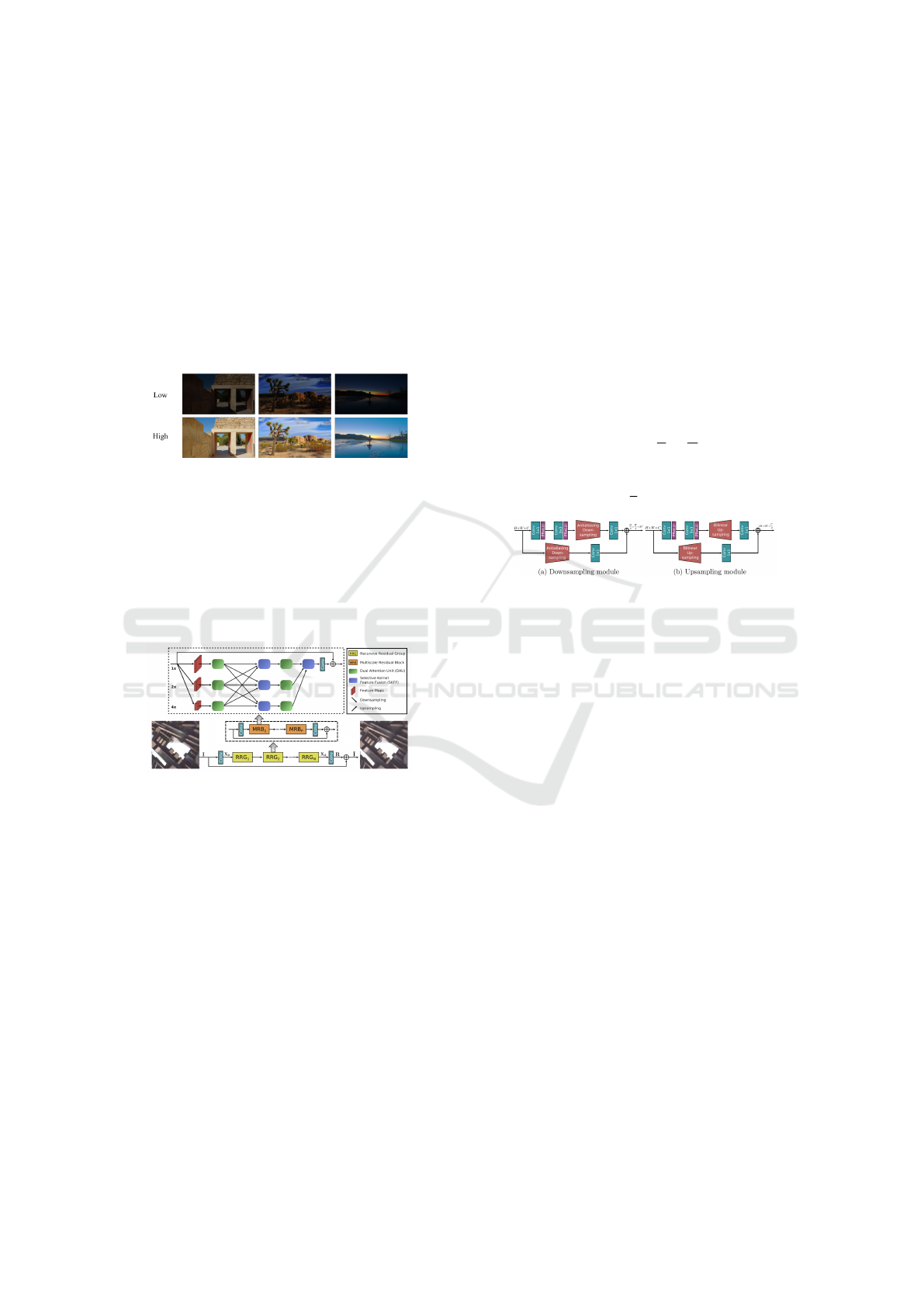
Figure 4: Example Images from LoL Dataset.

The SICE dataset contains 589 high-resolution se-

Using MIRNet for Low Light Image Enhancement

281

quences, with each sequence having multiple images

each with different levels of exposure. The SICE

dataset is split into two parts, the ﬁrst part containing

360 image sequences, and the second part containing

the rest. Due to limited resources, only the lowest

level of exposure for each image of the ﬁrst part of

this dataset was used. The training process remains

the same as the LoL dataset, with random crops of

128 by 128 generated before feeding the data to the

network. Likewise, 300 images were used for train-

ing, 185 images for validation, and 15 images for test-

ing.

Figure 5: Example images from SICE Dataset.

3.2 Model Selection and Architecture

MIRNet enhances images by utilizing a multi-scale

approach to address different levels of details in an

image (more on this later). MIRNet also employs a

residual design to allow for a much deeper architec-

ture(Zamir et al., 2003).

Figure 6: Overall Architecture of MIRNet.

When a colored image I of dimensions H × W × 3

is passed into MIRNet, it ﬁrst goes through a convo-

lution layer to extract low level features. The output,

, a feature map of dimensions H × W × C where

C is the number of channels, is then passed through

N recursive residual groups (RRGs) to obtain a deep

feature map X

of dimensions H × W × C. Next, X

is passed through a convolutional layer to obtain a

residual image R of dimensions H × W × C. Finally,

the residual image and the original image are concate-

nated via simple summation to obtain the output im-

age

I. Within each RRG, the incoming feature map X

is passed through a convolutional layer followed by P

multi-scale residual blocks (MRBs) and then another

convolutional layer to obtain a feature map, which is

then concatenated with the original X

to obtain fea-

ture map X

i+1

. (Zamir et al., 2003)

The MRB can mimic the visual cortex of humans

by maintaining multiple fully convolutional parallel

streams of different resolutions that exchange infor-

mation to generate an output which is both spatially

and contextually precise (see Figure 6 for detailed ar-

chitecture). (Zamir et al., 2003)

As can be observed in Figure 6, in the beginning

of the MRB and during information exchange, fea-

ture maps entering or exiting different streams must

be downsampled or upsampled to be consistent with

the resolution of each stream. The upsampling and

downsampling module used in the MRB can be ob-

served in Figure 7. In summary, in a downsampling

module, an incoming feature map M of dimensions

H × W × C goes through a series of layers and is con-

catenated with a skip connection to produce an output

feature map of dimensions

× 2C. Similarly,

an upsampling module takes in a feature map M of

dimensions H × W × C and outputs a feature map of

dimensions 2H × 2W ×

(Zamir et al., 2003).

Figure 7: Detailed image of up/down sampling modules.

In order to share information across streams, the

MRB uses a Dual Attention Unit (DAU). The DAU

can ﬁlter irrelevant features, sharing only the useful

information. The DAU consists of two parts: a Spa-

tial Attention (SA) branch and a Channel Attention

(CA) branch. In the end, the output of each branch is

concatenated and passed on (Zamir et al., 2003).

The SA branch can determine the inter-spatial re-

lationships in the incoming feature map M and re-

calibrate features in M. It does this by applying a

Global Average Pooling (GAP) layer and a Global

Max Pooling (GMP) layer to M and then concatenat-

ing the results to get a feature map f , with dimensions

H × W × 2. Next, f is passed through a convolution

and a sigmoid activation function to get a spacial at-

tention map

f . Finally, M is rescaled using

f and out-

putted from the SA branch (Zamir et al., 2003).

The goal of the CA branch is to determine the

inter-channel relationships and recalibrate M accord-

ingly. It uses a squeeze and excitation mechanism to

determine which channels are more important, and

which ones can be disregarded (a more detailed ex-

planation can be found here: (Pr

ove, 2017)). It does

this by passing the incoming feature map M through a

GAP layer and then two convolution layers followed

by a sigmoid activation function to get channel acti-

vations d. M is then rescaled using d and outputted

from the CA branch (Zamir et al., 2003).

BIOIMAGING 2025 - 12th International Conference on Bioimaging

282

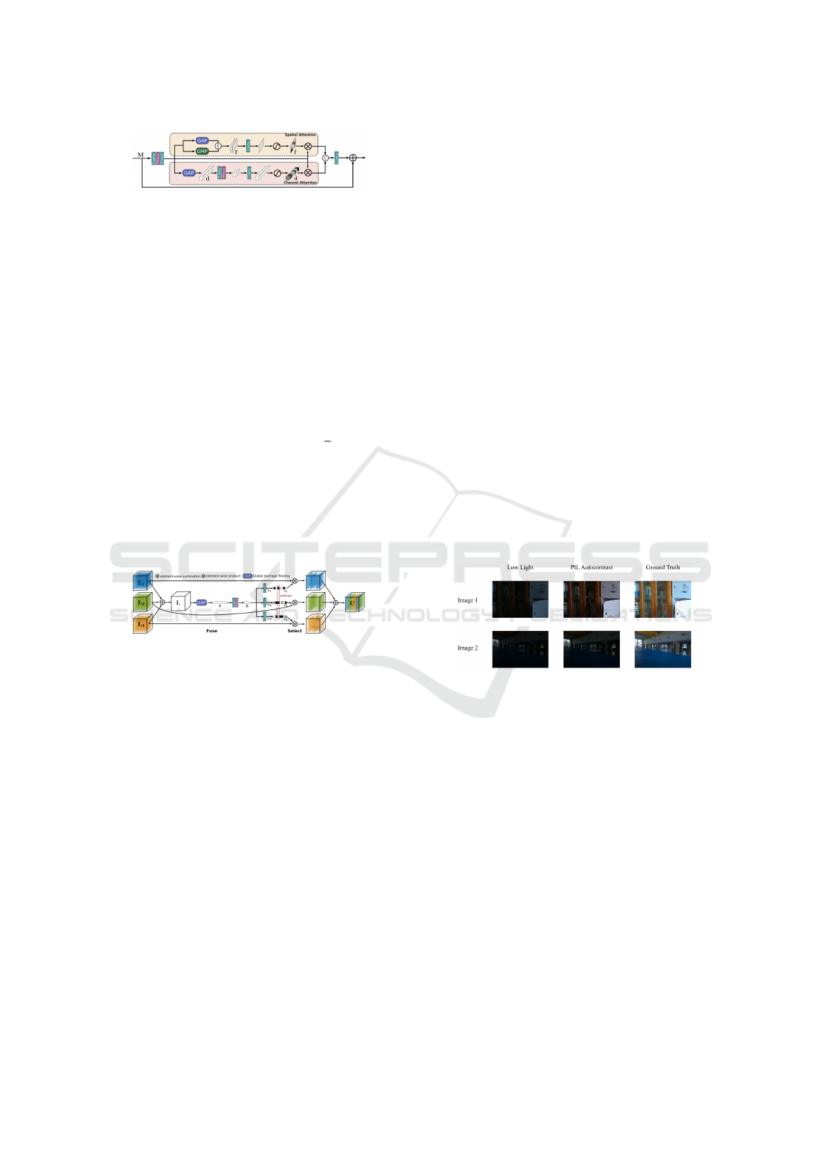
Figure 8: Detailed image of DAU block.

The last component of the MRB is the Selective

Kernel Feature Fusion (SKFF), which is responsible

for fusing features from multiple streams. It is able to

mimic a human’s visual cortex in that it can change

its receptive ﬁeld depending on the stimulus, by us-

ing feature aggregation and selection. The SKFF can

be divided into two parts: Fuse and Select. In the

Fuse section, the three incoming feature maps L

, L

and L

are concatenated via element-wise summation

to get the feature map L = L1 + L2 + L3. Next, L is

passed through a GAP layer to get channel wise statis-

tics of dimensions 1 × 1 × C, which is then passed

through a convolution layer to get compact channel

wise statistics z of dimensions 1 × 1 ×

. Finally, z

is passed through three parallel convolution layers to

get 3 channel descriptions v

, v

, and v

each of di-

mensions 1 × 1 × C. In the Select section, v

, v

, and

undergo a softmax activation to get attention acti-

vations s

, s

, and s

. Lastly, the output feature map

U is given by U = s

+ s

(Zamir et al.,

2003).

Figure 9: Detailed image of SKFF block.

3.3 Model Training Process

The model uses the Charbonnier Loss function and

the Adam Optimizer during the training process. By

default, the model runs with a batch size of four and

starts at a learning rate of 1e-4. It uses three RRGs,

with each RRG containing two MRBs, and the num-

ber of channels C of X

is set to 64. In each exper-

iment, only a few if not one hyper parameter were

modiﬁed to test its impact on the model’s perfor-

mance.

4 EXPERIMENTAL RESULTS

4.1 Experimental Setup

All experiments were run on Google Colab, which

runs on a Ubuntu OS and uses an Intel Xeon CPU

with 2 vCPUs and 13 GB of RAM, and a NVIDIA

Tesla K80 GPU with 12GB of VRAM.(Anonymous,

2023) The MIRNet code is written primarily using the

TensorFlow framework. TensorFlow provides many

useful features such as reading images and resizing

tensors. In addition, it allows the use of the Keras

API, which allows the user to easily build neural net-

work architectures with their built-in layers, such as

Convolution (Conv) 2d, Global Average Pooling 2d,

Global Max Pooling 2d, etc. The code also uses the

auto contrast feature from the PIL library as a baseline

to compare low light enhancement results of MIRNet

and this existing feature.

4.2 Performance Evaluation and

Analysis

The model is evaluated quantitatively using two main

methods: the loss function and the PSNR of the out-

put image. For each experiment, the minimum valida-

tion loss and maximum validation PSNR at any point

in the training process will be shared in this paper. In

addition, this paper also contains the overall trend of

the loss and PSNR during training, including both the

test and validation datasets. Finally, it also includes

two sample images from the LoL Dataset test set,

which can be interpreted qualitatively by the reader.

Figure 10: Two test images.

To start, here are the two images used throughout

the paper. PSNR of the PIL autocontrasted version of

each test image by comparing it with its correspond-

ing ground-truth image. The average PSNR of all 15

PIL autocontrasted images is about 11.2416.

4.2.1 Experiment 1

The ﬁrst experiment involves training the model with

the default hyper parameters, which, unsurprisingly,

yielded great results from the LoL dataset, as the

model has already been optimized greatly for the LoL

dataset. The minimum loss is 0.0983, and the maxi-

mum PSNR is 67.5981.

Using MIRNet for Low Light Image Enhancement

283

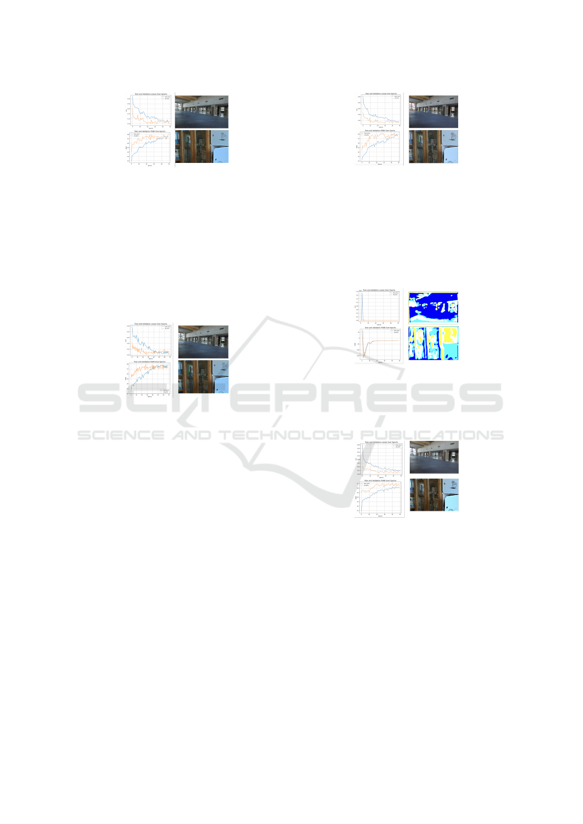
Figure 11: Experiment 1 Results.

4.2.2 Experiment 2

To test whether the model has completely plateaued,

the second experiment ran for 70 epochs. The results

are almost identical, with a minimum loss of 0.1016,

and a maximum PSNR of 67.8371, just marginally

greater than the previous, indicating that the model

has likely reached its full potential in just 50 epochs.

Judging by how little has changed, the rest of my ex-

periments on the LoL dataset were run on 50 epochs

to save resources.

Figure 12: Experiment 2 Results.

4.2.3 Experiment 3

Increasing the batch size from 4 to 8 caused the model

to crash during training due to a lack of memory.

4.2.4 Experiment 4

Increasing the random crop size from 128 by 128 to

256 by 256 caused the model to crash during training

due to a lack of memory.

4.2.5 Experiment 5

The Charbonnier loss function is really similar to the

root mean square error function, except it adds a small

constant to stabilize the training process. In this ex-

periment, the root mean square function is used in-

stead. The maximum PSNR for this experiment is

68.2198. Since the loss function is different compared

to the other experiments, it is unsuitable to use it as a

metric to evaluate the model’s performance in this ex-

periment compared to the other experiments.

Figure 13: Experiment 5 Results.

4.2.6 Experiment 6

An initial learning rate of 1e-3, yielded a minimum

loss of 0.1269 and a maximum PSNR of 65.4208.

However, these values are not representative of the

overall training curve. When excluding the ﬁrst two

epochs, a minimum loss of 2678.81 and maximum

PSNR of -20.8327 is the best the model can do.

Figure 14: Experiment 6 Results.

4.2.7 Experiment 7

An initial learning rate of 1e-5, yielded a minimum

loss of 0.1049 and a maximum PSNR of 67.083.

Figure 15: Experiment 7 Results.

4.2.8 Experiment 8 - 11

For each of these experiments, a change was made

to the model’s architecture. Since all 4 experiments

yielded similar results, the results are presented in a

table. Figure 16 is what the best performing experi-

ment looks like.

BIOIMAGING 2025 - 12th International Conference on Bioimaging

284

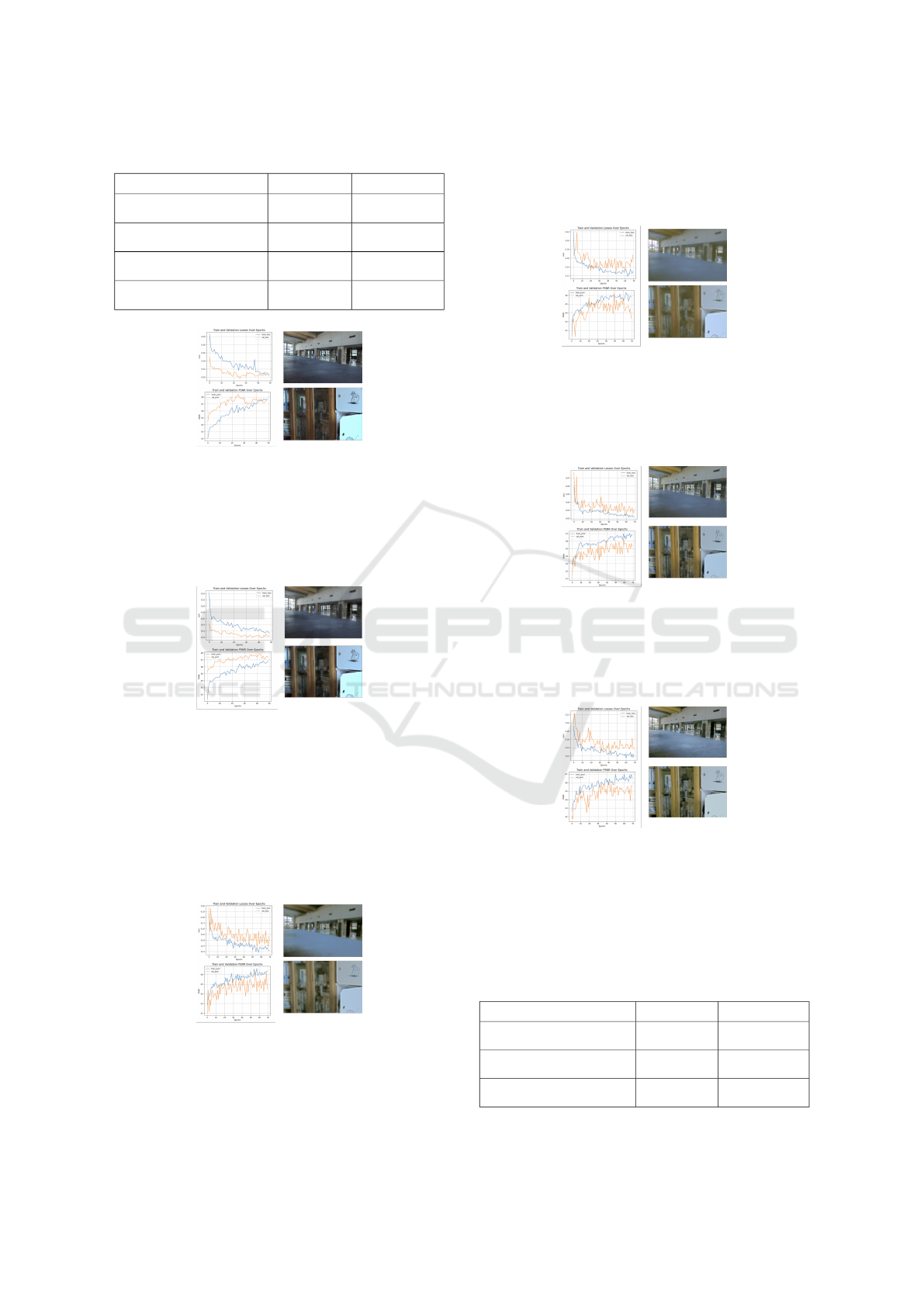
Table 1: Experiment 8 - 11 Results.

Change Minimum Loss Maximum PSNR

8. Increased the number of

MRBs per RRG by 1.

0.0965 68.3952

9. Changed the number of

channels of X0 to 32.

0.0977 68.1555

10. Changed the number of

channels of X0 to 96.

0.1009 67.8281

11. Added 1 parallel stream

to the SKFF

0.099 67.8437

Figure 16: Experiment 8 Results.

4.2.9 Experiment 12

Decreasing the number of RRGs and MRBs to 1

yielded a minimum loss of 0.1049 and maximum

PSNR of 67.083.

Figure 17: Experiment 12 Results.

4.2.10 Experiment 13

Moving on to the SICE Dataset, this experiment ran

for 70 epochs on the default values. The result of this

run shows a minimum loss of 0.1217 and a maximum

PSNR of 66.0102. Since the graph does not show an

obvious sign of a plateau, all subsequent experiments

were trained for 70 epochs.

Figure 18: Experiment 13 Results.

4.2.11 Experiment 14

An initial learning rate of 1e-5 yielded a minimum

loss of 0.1244 and a maximum PSNR of 66.3333.

Figure 19: Experiment 14 Results.

4.2.12 Experiment 15

Using root mean square loss, yielded a minimum loss

of 0.1217 and a maximum PSNR of 66.0102.

Figure 20: Experiment 15 Results.

4.2.13 Experiment 16

4 RRGs with 3 MRBs per, yielded a minimum loss of

0.1217 and a maximum PSNR of 66.3105.

Figure 21: Experiment 16 Results.

4.2.14 Experiment 17 - 19

The results of these three experiments are presented

in a table, as they are very similar. Figure 22 shows

the best performing run out of the three.

Table 2: Experiment 17 - 19 Results.

Change Minimum Loss Maximum PSNR

17. Decreased the number of

RRGs to 2.

0.1217 66.0889

18. Increased the number of

RRGs to 4.

0.1262 66.5826

19. Changed the number of

channels of X0 to 32.

0.1223 66.3105

Using MIRNet for Low Light Image Enhancement

285

Figure 22: Experiment 18 Results.

4.3 Discussion of Findings

The experiments yielded four key observations. First,

the loss and PSNR graphs for both training and val-

idation were less stable for the SICE Dataset com-

pared to the LoL Dataset. This instability is likely

due to the higher resolution of images in the SICE

Dataset, where a 128 × 128 crop may not be as rep-

resentative of the entire image as it would be for a

lower-resolution image. Second, the model’s learn-

ing rate must be carefully balanced; a rate too high

can cause overshooting, while a rate too low can re-

sult in the model getting stuck. Third, increasing the

complexity of the network does not necessarily lead

to better performance. This was unexpected, as it was

initially assumed that a more complex network, with

an increased number of weights, would yield superior

results. Lastly, architectural changes that have min-

imal impact on the model’s performance on the LoL

Dataset can signiﬁcantly affect its performance on the

SICE Dataset, particularly changes in the total num-

ber of MRBs and channels.

Overall, the model performed well on both

datasets. Achieving a PSNR value above 40, which is

generally considered good, demonstrates the model’s

strong performance.

5 CONCLUSION

5.1 Summary of Findings

Based on the quantitative and qualitative data, several

conclusions were drawn for both the LoL and SICE

Datasets.

For the LoL Dataset, it was observed that train-

ing for more than 50 epochs does not improve per-

formance, and doubling the batch size or increasing

the random crop size makes the model too resource-

intensive. Additionally, changing the loss function

from root mean square error to mean square error does

not enhance performance. The optimal initial learn-

ing rate was determined to be 1e-4. While increasing

the number of MRBs slightly improved performance,

other changes to the model’s architecture did not yield

signiﬁcant beneﬁts. However, decreasing the num-

ber of MRBs did worsen performance, though not as

much as initially expected.

For the SICE Dataset, training for more epochs led

to better performance, with the optimal initial learn-

ing rate also being 1e-4. Similar to the LoL Dataset,

changing the loss function had no impact on perfor-

mance. Increasing the number of MRBs provided a

slight improvement, but other architectural changes

tended to decrease performance.

5.2 Implications and Applications

Given MIRNet’s strong performance on the SICE

dataset, it has demonstrated versatility with numerous

potential real-world applications.

In photography and videography, MIRNet offers

a promising solution for improving image quality un-

der poor lighting conditions or low exposure. In the

domain of low light object detection, MIRNet could

enhance accuracy in settings such as nighttime envi-

ronments, which is crucial for automated driving and

surveillance. The results from the paper “Improving

the Accuracy of Object Detection in Low Light Con-

ditions using Multiple Retinex Theory-based Image

Enhancement Algorithms” by Aaryan Agrawal et al.

suggest MIRNet as a viable option for this task.

In archaeology and geology, MIRNet can address

the challenge of gathering prehistoric data in low light

environments, such as underground caves or man-

made tunnels, through low light image enhancement.

Similarly, MIRNet can be employed in underwater

exploration, where lighting conditions at great depths

are often poor, resulting in low-quality images. By

enhancing these images, MIRNet could enable sci-

entists to explore previously unreachable areas of the

ocean.

Lastly, in astrology, where celestial images may

be noisy or low quality due to the challenges of cap-

turing images from vast distances, MIRNet can pro-

vide higher quality images, aiding researchers in bet-

ter understanding the universe.

Note that data from each of these were not ex-

perimented with in the research, but judging by the

promising performance of the model on the SICE

dataset, it is reasonable to conclude that this per-

formance would not change given other low light

datasets.

5.3 Limitations and Future Work

The ﬁndings and observations in this article are not

exhaustive and much more remains to be explored.

However, due to time constraints and limited compu-

BIOIMAGING 2025 - 12th International Conference on Bioimaging

286

tational resources, only a limited number of experi-

ments were conducted for each parameter, which may

not be sufﬁcient to draw conclusions. Therefore, the

conclusions in this paper should be viewed as a gen-

eral guide for optimizing MIRNet’s architecture.

Several aspects could not be tested due to resource

and time limitations. These include exploring every

combination of four or fewer RRGs, four or fewer

MRBs, and two to four parallel streams; testing more

intermediate values for parameters such as batch size,

crop size, and number of channels; and experiment-

ing with additional low-exposure datasets focused on

speciﬁc tasks, such as underwater images, security

footage, celestial objects, or human faces.

Despite these limitations, MIRNet’s strong perfor-

mance on alternative datasets suggests it could be a

powerful tool in the future of AI technology, with sig-

niﬁcant potential for real-world applications.

REFERENCES

Nanos, G. (2023). Neural networks: Pooling layers. Bael-

dung.

Agrawal, A., Jadhav, N., Gaur, A., Jeswani, S., and Kshir-

sagar, A. (2022). Improving the accuracy of object de-

tection in low light conditions using multiple retinex

theory-based image enhancement algorithms. IEEE

Xplore.

Anonymous (2023). Whats the hardware spec for google

colaboratory. Saturn Cloud.

LeCun, Y., Bengio, Y., and Hinton, G. (2015). Deep learn-

ing. Nature.

Parmar, R. (2018). Training deep neural networks. Towards

Data Science.

ove, P.-L. (2017). Squeeze-and-excitation networks. To-

wards Data Science.

Zamir, S., Arora1, A., Khan, S., Hayat, M., Khan, F., Yang,

M., and Shao, L. (2003). Learning enriched features

for real image restoration and enhancement. Springer.

Using MIRNet for Low Light Image Enhancement

287