ML-Based Virtual Sensing for Groundwater Monitoring in the

Netherlands

Laure Grisez

, Shreshtha Sharma

and Paolo Pileggi

Applied Mathematics, ENSTA Paris, France

Advanced Computing Engineering, TNO, The Netherlands

Keywords: Machine Learning, Groundwater Monitoring, Virtual Sensors, Gaussian Process Regression,

Graph Neural Networks, Spatial Interpolation.

Abstract: The increasing need for effective groundwater monitoring presents a valuable opportunity for Machine

Learning (ML)-based virtual sensing, especially in regions with challenging sensor networks. This paper

studies the practical application of two core ML models, Gaussian Process Regression (GPR) and Position

Embedding Graph Convolutional Network (PEGCN), for predicting groundwater levels in The Netherlands.

Additionally, other models, such as Graph Convolutional Networks and Graph Attention Networks, are

mentioned for completeness, offering a broader understanding of ML methods in this domain. Through two

experiments, sensor data reconstruction and virtual sensor prediction, we consider model performance, ease

of implementation, and computational requirements. Practical lessons are drawn, emphasising that while

advanced models like PEGCN excel in accuracy for complex environments, simpler models like GPR are

better suited for non-experts due to their ease of use and minimal computational overhead. These insights

highlight the trade-offs between accuracy and usability, with important considerations for real-world

deployment by practitioners less familiar with ML.

1 INTRODUCTION

Groundwater monitoring is essential for sustainable

water resource management, particularly in countries

like The Netherlands, where precise groundwater data

supports flood control, irrigation, drinking water

supply, and environmental protection.

Traditional monitoring approaches rely heavily on

physical sensor networks, which are costly and often

impractical to deploy and maintain due to logistical,

legal, and geographic constraints. This has opened up

a significant opportunity for Machine Learning (ML)-

based virtual sensing systems to predict groundwater

levels in regions where physical sensors are lacking,

improving monitoring coverage and operational

efficiency.

This paper presents an investigation into the

practical application of two relevant ML models for

virtual groundwater level sensing, namely Gaussian

Process Regression (GPR) and Position Embedding

Graph Convolutional Network (PEGCN).

https://orcid.org/0009-0001-6031-201X

GPR is well-known for its ability to model spatial

correlations and estimate uncertainty, making it a

strong candidate for environments where predictive

reliability is critical. PEGCN, by contrast, employs a

graph-based framework enhanced with positional

encoding, allowing it to better capture complex

spatial relationships in sensor networks. This study

aims to evaluate the strengths and weaknesses of

these models in terms of their performance,

scalability, and adaptability to groundwater

monitoring needs.

In addition to GPR and PEGCN, we also mention

other models, including Graph Convolutional

Networks (GCN) and Graph Attention Networks

(GAT). These models are mentioned to provide a

holistic view of available ML techniques for spatial

interpolation tasks. This exploration allows us to

learn valuable lessons, particularly concerning their

readiness for use in practical situations by non-expert

users, such as water resource managers or

environmental engineers with limited ML expertise.

Grisez, L., Sharma, S. and Pileggi, P.

ML-Based Virtual Sensing for Groundwater Monitoring in the Netherlands.

DOI: 10.5220/0013101100003890

Paper published under CC license (CC BY-NC-ND 4.0)

In Proceedings of the 17th International Conference on Agents and Artiﬁcial Intelligence (ICAART 2025) - Volume 3, pages 175-184

ISBN: 978-989-758-737-5; ISSN: 2184-433X

175

Beyond performance metrics like accuracy, this

paper highlights crucial practical considerations such

as ease of implementation, computational

complexity, and the resource demands associated

with each model. These factors are essential for real-

world applications, as they determine the feasibility

of adopting ML models in routine groundwater

monitoring tasks. This study provides insights into

the trade-offs between model accuracy and practical

usability, helping guide model selection based on

specific geographic conditions, operational

requirements, and user expertise.

The remainder of the paper is organised as

follows: Section 2 provides background on

groundwater monitoring and the ML techniques

considered. Section 3 reviews related work. Section 4

presents the case study, implementation details, and

experimental results. Section 5 discusses the lessons

learned and concludes with potential directions for

enhancing ML-based virtual sensing systems in

groundwater monitoring.

2 BACKGROUND

2.1 Groundwater Level Measurement

Groundwater level measurement provides crucial

insights into subsurface water dynamics, particularly

in The Netherlands, where effective water

management is vital due to its low-lying geography

and high population density. Integrating ML with

sensor data enables more accurate spatial and

temporal interpolation, improving predictions in

unmonitored areas.

ML-based virtual sensors exploit real-world data

from sensor networks to estimate groundwater levels

where direct measurements are unavailable.

Typically installed in boreholes, these sensors record

water levels continuously, helping to understand

seasonal variations and human impacts. In regions

with sparse networks, ML models fill gaps using

historical sensor data, even when some sensors have

missing or incomplete records.

In The Netherlands, various organisations manage

groundwater sensor networks, with platforms like the

Dutch Hydrological Information Platform (HYDAP)

offering access to real-time and historical

groundwater data. These platforms collect, store, and

analyse sensor measurements, providing valuable

data for researchers, policymakers, and engineers.

Users can access sensor data through APIs or web

portals, enabling integration with analytical tools for

data analysis and modelling.

ARGUS is another such a platform developed by

Aveco De Bondt. It plays a significant role in

groundwater monitoring across the country. The

platform is designed to support waterboards,

municipalities, and drinking water companies by

aggregating and analysing groundwater data from a

wide network of sensors deployed across the country.

This platform monitors these water levels in real-

time, enabling more informed decision-making for

flood control, water management, and environmental

protection. Using advanced data visualisation and

predictive analytics, it helps assess trends, manage

risks, and optimise water strategies by integrating

data from diverse sources, like local sensors and

national datasets. This enhances operational

efficiency in water management, offering insights for

both immediate actions and long-term planning.

Groundwater monitoring is uniquely challenging

due to its slow response to external factors compared

to surface water. For readers interested in a more

comprehensive understanding of groundwater

monitoring techniques, including sensor systems and

hydrological modelling, we recommend the

consulting a popular text (Rothman, 2021).

2.2 Gaussian Process Regression

Primer

GPR is a non-parametric, Bayesian approach to

regression that is particularly useful for modelling

complex, multi-dimensional datasets. It is preferred

in geospatial analysis and environmental modelling

due to its ability to provide a probabilistic framework

and quantify the uncertainty in predictions for making

informed decisions in these fields.

It models the observed data 𝑦 at locations 𝑋 using

a Gaussian process (GP), which is a collection of

random variables, any finite number of which have a

joint Gaussian distribution.

A GP is fully specified by its mean function m





and covariance function 𝑘



𝑥, 𝑥





. Typically, m





taken as zero, and the focus is on the choice of the

covariance function 𝑘



𝑥, 𝑥





, also known as the

kernel, which encodes assumptions about the function

to be learned.

The kernel function determines the shape of the

covariance between pairs of points in the input space.

A popular choice for capturing varying degrees of

smoothness in the underlying function is the Matérn

kernel, where 𝑉 controls the smoothness of the

function. 𝑉 allows the kernel to interpolate between

different levels of smoothness. E.g., when 𝑉=0.5, it

reduces to the exponential kernel, producing less

smooth functions. As 𝑉 increases, the resulting

ICAART 2025 - 17th International Conference on Agents and Artiﬁcial Intelligence

176

functions become smoother, with the kernel

converging to the squared exponential kernel as 𝑉→

∞.

GPR is well-suited for environmental modelling

and geospatial analysis. Its flexible kernel function

can be customised to fit diverse data types and

structures. As a non-parametric method, it adapts to

complex data patterns without requiring predefined

models. For readers seeking to explore the theory and

applications of GPR in depth, (Rasmussen, 2006)

provides comprehensive coverage.

2.3 Deep Learning for Spatial

Reconstruction

Deep Learning (DL) has significantly advanced the

field of ML. There are powerful tools to model

complex data structures and extract meaningful

patterns. Among the various architectures,

Transformer architectures and Graph Neural

Networks (GNN) have emerged as particularly

influential for handling structured data, especially in

spatial reconstruction tasks.

Transformers, introduced by (Vaswani, 2017),

represent a breakthrough in sequence modelling that

has since been adapted for a wide range of tasks

beyond natural language processing. The

Transformer’s self-attention mechanism allows the

model to weigh the influence of different parts of the

input data, particularly useful for modelling

sequential data where the context and order of data

points are crucial.

On the other hand, GNNs are powerful tools for

learning representations of nodes and edges within a

graph. These representations are refined by

aggregating information from neighbouring nodes

and edges, enabling the model to propagate

information effectively across the entire graph.

Unlike traditional neural networks, GNNs use the

graph structure during learning. This is especially

beneficial for spatial data where the relationships

between data points are determined by their

connectivity, rather than merely by their order or

proximity. They are highly flexible and adaptable,

capable of handling various types of graphs,

including directed, undirected, weighted, and multi-

relational graphs. This makes them suitable for a

broad range of applications, from analysing

molecular structures to understanding dynamics

within social networks.

In spatial reconstruction, GNNs have been used to

model physical processes where data is naturally

represented as a network of interconnections, e.g.,

river networks, road networks. They have been

employed to predict traffic flow, model water

distribution in rivers, and simulate the spread of

pollutants in air or water networks. By using GNNs,

researchers can incorporate both the spatial

arrangement and the physical or functional

connectivity between data points, leading to more

accurate and context-aware predictions.

Recent research has explored combining

Transformer architectures with GNNs to exploit the

self-attention mechanism's ability to process

sequential dependencies and GNNs’ capacity to learn

from graph-structured data. This hybrid approach is

particularly potent for spatio-temporal data, where

both the temporal dynamics and the spatial

connections must be understood and modelled

effectively.

One of the promising applications of this hybrid

approach is in environmental science, where models

need to capture complex interactions over both time

and space, such as the evolution of weather patterns,

the spread of contaminants, or the changes in

groundwater levels. By integrating Transformers with

GNNs, models can better capture the multifaceted

nature of these processes, leading to more accurate

predictions and deeper insights into the underlying

phenomena. For detailed elaborations on graph

representation learning and transformer architectures,

interested readers are referred to the respective works

of (Rothman, 2021; Hamilton, 2020).

3 RELATED WORK

Groundwater level prediction research features the

study of various ML techniques, ranging from

traditional methods to cutting-edge DL models.

Classical regression methods, such as GPR and

Sparse Identification of Nonlinear Dynamics

(SINDy), have been foundational in spatial prediction

tasks related to groundwater levels.

GPR, known for its ability to model continuous

spatial relationships and estimate uncertainties, has

proven useful, although it faces computational

challenges with large datasets due to its complexity

(MacKay, 1998; Gu, 2012). SINDy, on the other

hand, is adept at capturing complex spatial dynamics

and nonlinear dependencies but is less effective for

direct value prediction (Brunton, 2015; Castro-Gama,

2022).

Ensemble methods, like Random Forest, have

been applied to model topological and flow dynamics

within water networks. These methods handle time

dependencies with fewer parameters and are effective

for capturing flows across a network’s edges, while

ML-Based Virtual Sensing for Groundwater Monitoring in the Netherlands

177

typical prediction tasks focus on node values (Sun,

2019; Ahmadi, 2019).

DL, especially models, such as Convolutional

Neural Networks (CNN), Long Short-Term Memory

(LSTM) networks, Transformer models, and Graph

Neural Networks (GNN), have significantly

advanced spatial and temporal data modelling in

water distribution networks (Paepae, 2021). GNNs,

particularly their extensions, like Graph Attention

Networks (GAT) and Temporal GNNs (T-GNNs), are

well-suited for modelling complex network structures

with nodes and edges, enabling more accurate

predictions of dynamic processes, such as water

distribution (Truong, 2024; Zhao, 2019; Veličković,

2018).

Scalability issues often arise with GNNs due to

their high computational demands and numerous

parameters (Topping, 2022; Zheng, 2024). To address

this, innovative techniques like Position Embedding

Graph Convolutional Network (PEGCN) and

Nodeformer have been developed (Chamberlain,

2021; Wu, 2022). These models handle challenges

such as over-squashing, heterophily, and long-range

dependencies by incorporating positional encoding,

making them effective for spatial interpolation tasks

like groundwater level prediction. Nodeformer uses

Transformer architectures to improve the scalability

and performance of graph-based models, although it

requires higher computational resources.

Hybrid models have also been explored, e.g.,

combining GNNs with LSTMs or CNNs, to enhance

prediction robustness by capturing dynamic temporal

and spatial changes in water levels (Lu, 2020; Nasser,

2020). Moreover, probabilistic spatio-temporal graph

models, such as DIffSTG, and attention-based

models, like spatial-temporal attention mechanisms,

have been developed to improve prediction accuracy

and reliability, surpassing traditional methods in

several aspects (Shi, 2021; Wen, 2023). These

methods are particularly useful in environmental

science, where models must capture both the spatial

and temporal dynamics of water systems.

Fast downscaling methods, such as CNN-based

approaches, have also been employed to improve data

resolution in environmental predictions. While

statistical techniques, like quantile perturbation, have

been explored, DL methods have outperformed

traditional models in capturing complex temporal

features for downscaling tasks (Tabari, 2021; Sun,

2024). These advancements demonstrate the potential

of ML models, particularly those incorporating

spatial and temporal dynamics, for more accurate

groundwater level predictions.

The growing applicability and use of ML

techniques, from classical regression to advanced

GNN architectures, continues to improve water level

prediction. PEGCN, with its positional encoding,

exemplifies these advancements, offering enhanced

spatial awareness for groundwater level prediction. A

challenges lies in integrating temporal dynamics and

refining these models for broader applicability in

water resource management.

4 INVESTIGATIVE STUDY

This study aims to estimate groundwater levels across

Schiedam, Netherlands, using real sensor data.

Schiedam’s complex clay terrain and urban

infrastructure create significant variability in

groundwater levels. The dataset, from the ARGUS

platform, includes hourly measurements from 151

sensors over 7.6 years (66,921 hours), with water

levels ranging from -2.8m to 0.3m. For efficiency, the

analysis focuses on the last 60 days of data.

ML models are used to generate virtual sensor

values, enhancing spatial coverage without the cost of

additional physical sensors. These virtual sensors

predict levels in unmonitored areas by utilising spatial

correlations from the data. The dataset pairs sensor

readings with geographic coordinates, labelling

missing or target data as ‘virtual’ to allow for model

training and accurate predictions. Schiedam’s

environment is a challenging representative test case

for virtual sensing technologies in groundwater

monitoring.

4.1 Model Implementation and Testing

The dataset includes hourly groundwater level

readings from multiple sensors, accompanied by the

geographic coordinates of each sensor. If a sensor is

missing data at certain timestamps or is flagged for

prediction, the entry is labelled as ‘virtual,’ and the

corresponding value is set to zero for prediction

purposes.

The dataset is chronologically ordered by

timestamp, with each timestamp representing a

snapshot of sensor readings. For graph-based models,

like the PEGCN, a k-nearest neighbours (kNN) graph

is constructed from these snapshots using the

Euclidean distances between sensor coordinates.

For statistical regression approaches, such as

GPR, both the sensor values and coordinates are

normalised to improve the accuracy of the model’s

predictions.

ICAART 2025 - 17th International Conference on Agents and Artiﬁcial Intelligence

178

4.1.1 Handling Missing Data and Virtual

Sensors

Two distinct approaches are used to handle missing

data and virtual sensors, namely dynamic graph (with

node removal) and fixed graph (with zero-filling).

Dynamic Graph Approach: Missing data is

excluded from the input, and the model generates a

regression without receiving any information about

the missing sensor. This method works best for

spatially-aware models, like GPR and PEGCN.

For GPR, the model does not rely on graph

structures and can function effectively with masked

data. In the case of PEGCN, however, removing

nodes results in the need to reconstruct a new graph

at each iteration, which can reduce the model’s ability

to maintain a constant graph structure. However, this

dynamic input graph could make the model more

adaptable when predicting new virtual sensors

without requiring a complete retraining of the model.

Fixed Graph Approach: The graph structure

remains constant and missing data is replaced with

zeros during both training and testing. The loss is

computed only between the output predictions and the

actual values of the existing sensors.

Graph-based models, like PEGCN and other

GNNs trained with this method, tend to perform

better at reconstructing the sensor network when the

virtual sensors are predetermined. However, this

approach may perform poorly when asked to predict

out-of-distribution sensors, i.e., sensors that were not

part of the initial training set.

4.1.2 Model Training and Testing

During model training, PEGCN and other GNN

algorithms randomly mask half of the sensor inputs,

setting their values to zero, while still incorporating

them into the loss function. This masking technique,

applied to batches of snapshots, enables the model to

predict missing sensor values by leveraging the

available data from other sensors. This method

enhances the model’s understanding of spatial

dependencies between sensors.

In contrast, training the GPR model involves

optimising two key hyperparameters, i.e., the

constant value and the length scale that control the

smoothness and variability of predictions. The model

is fine-tuned by minimising prediction errors, to

capture spatial correlations in the predictions.

The testing phase mirrors the training setup. For

GNN-based models like PEGCN, we reconstruct the

masked sensor values and compare them with actual

data. GPR, on the other hand, directly predicts

groundwater levels based on learned spatial

correlations. Both models are evaluated using

standard error metrics like Mean Absolute Error

(MAE) and Root Mean Square Error (RMSE).

4.2 Experimental Setup

The study is designed to evaluate the models’ ability

to learn from real sensor data and predict groundwater

levels. Two main experiments were conducted to

assess both the reconstruction of known sensors and

the prediction of virtual sensors in unmonitored areas.

The first experiment (Experiment 1) focuses on

evaluating the models’ ability to understand and

reconstruct the dynamics of the existing sensor

network. This is particularly important for DL

models, like PEGCN and GATRes, as GPR does not

require training and thus has limited capacity to

capture network dynamics.

To conduct this experiment, the dataset is divided

into two parts: The first 40 days of data are used for

training, while the last 20 days are reserved for

validation. During training, in each snapshot, half of

the sensors are randomly masked, and the models are

trained to predict the values of the masked sensors

based on the available data from the other sensors.

In the evaluation phase, the same procedure is

applied: Half of the sensors are masked, and the

model predicts the values for these masked sensors.

The predicted values are then compared to the actual

sensor readings to compute the error.

The second experiment (Experiment 2) is

designed to directly assess the models’ ability to

predict the values of virtual sensors, aligning with the

ultimate goal of creating virtual sensors to extend the

spatial coverage of the network.

One sensor is selected as the target for error

calculation, and this sensor is masked in all the

snapshots during training. The training process is

similar to Experiment 1, except the loss is computed

on all nodes apart from the chosen sensor, ensuring

that the model never receives any direct information

about the target sensor.

During evaluation, all sensor data excluding the

target sensor are fed into the model. Only the

coordinates and a value of zero are provided for the

target sensor. The model is then required to predict

the target sensor’s value, and the error is computed

based on this prediction.

In these experiments, the following models were

evaluated:

Mean Model: Used only in Experiment 1, this

simple baseline model outputs the mean value of each

sensor calculated from the training dataset. It serves

ML-Based Virtual Sensing for Groundwater Monitoring in the Netherlands

179

as a control for comparison with more complex

models.

GPR: Uses a Matérn kernel with V = 3/2, a fixed

length scale of 1, and a constant value of 5. This

version of GPR does not undergo optimisation.

GPR (Optimised): Also uses a Matern kernel

with V = 3/2, but both the length scale and constant

value are optimised to minimise prediction errors on

the training dataset.

GCN and PEGCN: Trained for 100 epochs, with

a learning rate of 0.001, weight decay of 0.0001, and

batches of 64 snapshots. The loss function is Mean

Square Error (MSE), and a kNN graph is constructed

with k = 4. For PEGCN, both a version with a

constant graph structure and one without are trained.

GATRes: Trained for 200 epochs, with a learning

rate of 0.01, weight decay of 0.00001, and batches of

64 snapshots. Like PEGCN, the loss function is MSE,

and kNN graphs are created with k = 4.

We expect GATRes, with its higher number of

parameters, will perform well in the sensor

reconstruction task, i.e., Experiment 1. However,

PEGCN and GPR may outperform GATRes in the

virtual sensor prediction task, i.e., Experiment 2, due

to their ability to capture spatial relationships and

their geographical awareness.

The models performance are gauged using MSE

as the loss function during training, MAE for

effectiveness, and RSME to measure overall

prediction accuracy.

Our evaluation extends beyond these performance

metrics to include other key factors, such as ease of

implementation, which we rate as simple, moderate,

or hard, based on the complexity of running the code

and integrating data.

We also assess resource complexity by

considering training time and prediction time. These

dimensions help illustrate the trade-offs between

model effectiveness and computational demands.

4.3 Results

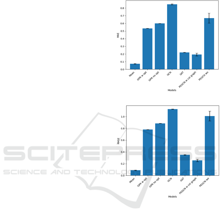
Figures 1 and 2 present the performance results for

each model in Experiment 1, showing the MAE and

RMSE, respectively. The figure shows that the simple

mean function outperformed all other models in terms

of both MAE and RMSE, which was somewhat

unexpected.

Figure 1: MAE for each model in Experiment 1.

Figure 2: RMSE for each model in Experiment 1.

This result can be attributed to the relatively stable

groundwater levels in the study area, where values do

not fluctuate significantly over time due to the

controlled nature of the environment. As a result, a

model outputting constant mean values is sufficient

for reconstructing the missing data, which explains

why the mean model performed so well in this

context.

Among the more complex models, PEGCN and

GATRes exhibited the best performance in

reconstructing the sensor network. However, they did

not outperform the mean model.

The potential for improvement lies in their ability

to learn more intricate patterns from the data.

However, the models’ difficulty in handling the

largely static nature of the groundwater data could

have hindered their performance.

ICAART 2025 - 17th International Conference on Agents and Artiﬁcial Intelligence

180

Adjustments such as normalising the data per

sensor or imputing missing values with the mean

instead of zeros may help reduce confusion within

these models and improve their results. PEGCN with

a constant graph structure showed better results than

the version with a dynamic graph, confirming the

importance of maintaining the network structure for

spatial data reconstruction.

Interestingly, GPR models, despite being less

complex and requiring no training, performed

surprisingly well, outperforming two of the DL

models, namely the GCN and PEGCN without a

constant graph. This suggests that GPR, with its

strong spatial correlation modelling, is able to handle

such data effectively. The model’s ability to make

accurate predictions without learning from the full

sensor network is particularly promising for virtual

sensor prediction tasks.

None of the models exceeded the mean function

in this particular case, but PEGCN and GATRes

showed potential when provided with additional

features and improved data handling methods. GPR

models’ performance demonstrates that simpler

methods may be effective when spatial correlations

are present, making them useful for tasks like virtual

sensor prediction.

Positional encoding within GCN significantly

improved its regression capabilities, even when

competing against more parameter-rich models, like

GATRes. These results highlight the need for further

refinement, particularly in handling static

environments, and suggest that GPR can serve as a

baseline for future virtual sensor prediction

experiments with an expected error of approximately

50cm.

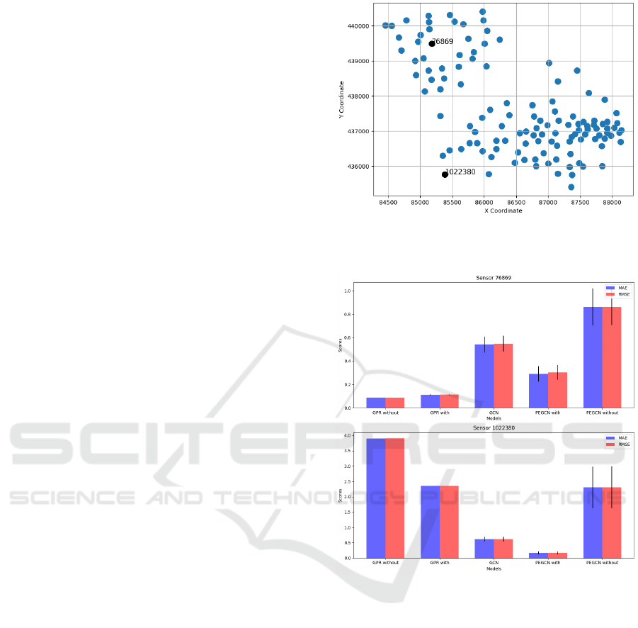
Figure 3 shows the cartesian plot of sensors

#76869 and #1022380. As you can see, these were

selected in two seemingly distinct clusters, in

respective central and peripheral positions.

In Experiment 2, the models’ performance varied

significantly depending on the sensor being predicted.

As shown in Figures 4 through 8, PEGCN generally

produced more stable results across different sensors,

with errors ranging from 20cm to 2m.

In contrast, GPR exhibited much greater

variability in its predictions. As shown in Fig. 4, GPR

performed well on sensor #76869 reaching 10cm, but

its error for sensor #1022380 reached nearly 4m.

Figure 3: Cartesian plot of sensors #76869 and #1022380

from Experiment 2.

Figure 4: MAE and RSME (in metres) for each method

and sensors #76869 (top) and #1022380 (bottom) in

Experiment 2.

This disparity can be explained by GPR’s

limitations when reconstructing sensors that are either

geographically distant from other sensors or have

values that differ greatly from their neighbours. Its

inherent spatial correlation modelling is highly

sensitive to the distance between sensors, making it

less effective in regions where the groundwater levels

fluctuate significantly across short distances or where

the data distribution is irregular.

PEGCN, with its positional encoding and graph-

based structure, appears to be better equipped to

handle such discrepancies, allowing it to maintain

more consistent performance even with sensors that

exhibit varying behaviours.

ML-Based Virtual Sensing for Groundwater Monitoring in the Netherlands

181

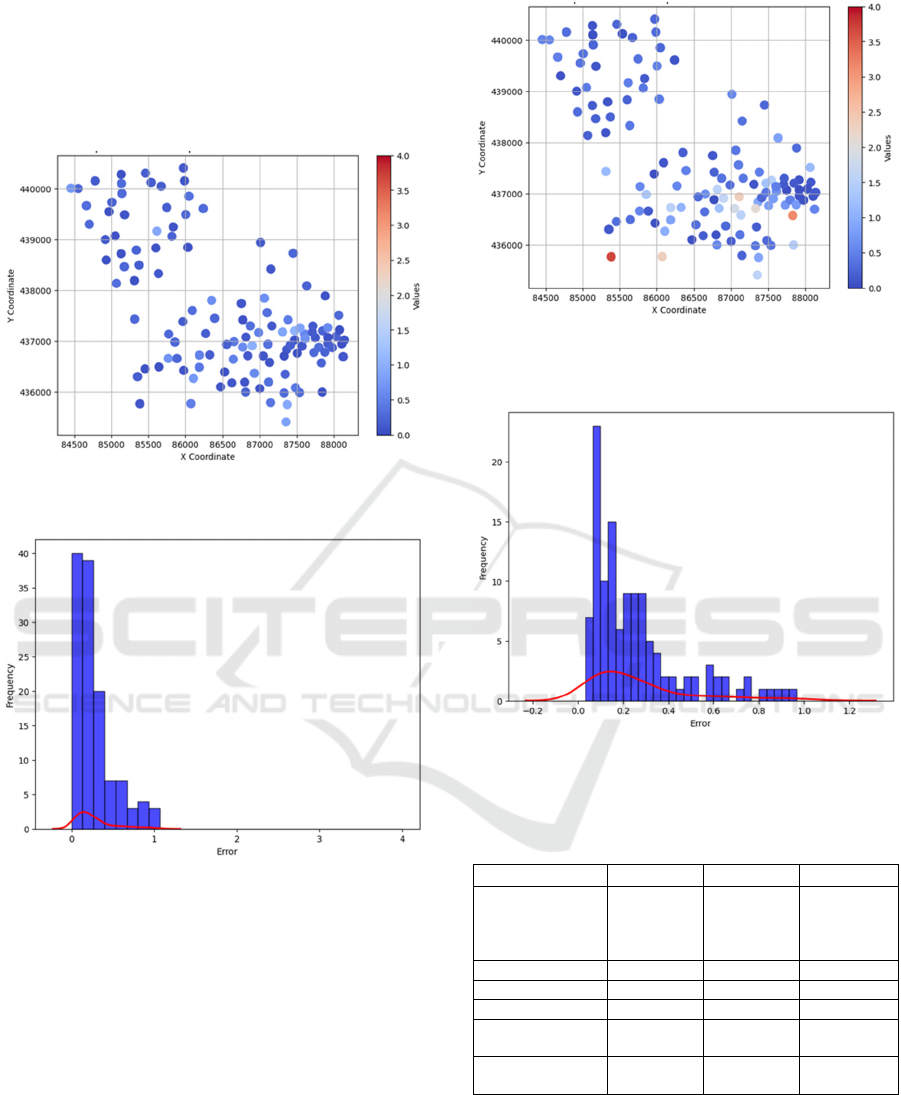
MAE error distributions shown in Fig. 8, suggests

that GPR struggles with outliers, especially in cases

where the sensor’s value is far from its neighbouring

sensors. This indicates that GPR’s interpolation

capabilities are less robust in areas with extreme

values or isolated sensors.

Figure 5: MAE PEGCN per-sensor performance (in metres)

in Experiment 2 (RMSE not shown due to similar values).

Figure 6: MAE distribution PEGCN performance (in

metres) in Experiment 2 (RMSE not shown due to similar

values).

On the other hand, PEGCN’s stability across the

sensor network demonstrates the advantage of

maintaining a graph structure that captures

geographic relationships more accurately.

Experimenting with kernel functions and

hyperparameters could potentially improve GPR’s

performance, particularly in areas with highly

variable levels. However, GPR seems less suited for

environments where significant differences exist

between nearby sensors.

Figure 7: MAE GPR (without optimisation) per-sensor

performance (in metres) in Experiment 2 (RMSE not shown

due to similar values).

Figure 8: MAE distribution GPR (without optimisation)

performance (in metres) in Experiment 2 (RMSE not shown

due to similar values).

Table 1: Other factors results for GPR, PEGCN, and GCN.

Factor GPR PEGCN GCN

Prediction

Snapshot

0.03s

Dataset

22.32s

Snapshot

0.35s

Dataset

59.52s

Snapshot

0.34

Dataset

56.94s

Training 10:42.4 01:37.0 00:53.6

evice CPU GPU GPU

No. parameters 2 6521 1153

Ease of

implementation

Simple Moderate Moderate

Time to

completion

Day Week Week

While PEGCN exhibits better stability and

performance for virtual sensor prediction in areas

with complex sensor networks, GPR still provides a

valuable baseline with reasonable accuracy,

especially when spatial relationships are consistent.

However, both models could benefit from further

ICAART 2025 - 17th International Conference on Agents and Artiﬁcial Intelligence

182

optimisation and testing in different environments to

fully understand their capabilities and limitations.

Beyond performance metrics such as prediction

accuracy, other important factors must be considered

when comparing models. Specifically, ease of

implementation and resource complexity, are among

those reported in Table 1. These aspects can

significantly impact the practicality of a model for

real-world applications.

Among the models, GPR stands out for its

simplicity. GPR is relatively easy to implement, as it

does not require extensive training, and its

performance remains stable with well-chosen initial

parameters. This makes GPR an ideal choice for

applications where ease of use and minimal

computational overhead are priorities. Additionally,

GPR runs efficiently on standard CPUs, making it

accessible for smaller datasets or less resource-

intensive tasks.

However, one major limitation is its scalability.

As the number of sensors increases, GPR’s

computational complexity grows cubically, which

can lead to performance bottlenecks with larger

datasets.

In contrast, PEGCN and GCN are more

challenging to implement. They require a solid

understanding of graph-based neural networks and

experience with libraries, like PyTorch Geometric.

Setting up these models involves more intricate input

preparation and parameter tuning, particularly for the

graph structure and embeddings. Moreover, these

models perform best on GPUs, meaning access to

high-performance hardware is crucial for their

implementation and training, especially when dealing

with larger datasets.

During the study, Nodeformer was also explored

as a potential model. However, it was ultimately

unsuccessful in our case, highlighting the difficulty of

adapting advanced DL models to specific tasks. This

illustrates the inherent challenge in implementing

cutting-edge models, which may not always be ready

for practical applications without significant

customisation.

Table 1 also provides an overview of the resource

demands of each model in terms of prediction time,

training time, and ease of implementation. It reveals

that GPR is the most resource-efficient, with a

prediction time of just 0.021965s per snapshot and no

need for training on large datasets.

PEGCN and GCN are significantly more

demanding, with training times for the whole dataset

reaching over an hour and requiring substantial GPU

resources. Additionally, GATRes and Nodeformer

were not fully implemented due to their high

complexity, suggesting that these models may not be

easily used in environments where computational

resources are limited.

As the table shows, GPR is the fastest and

simplest to implement, making it ideal for small-scale

applications with minimal training requirements.

However, PEGCN performs better in terms of

accuracy and stability for virtual sensor

reconstruction tasks, although it demands more data,

training time, and computational resources. The need

to retrain PEGCN whenever new virtual sensors are

added increases its complexity, both in terms of data

management and coding effort.

5 CONCLUSION

A key takeaway is the importance of comparing

available ML models based on their performance, as

well as on their suitability for practical applications.

We investigated models like GPR, PEGCN, and GCN

for groundwater level monitoring, with a focus on

real-world implementation and usability. This focus

is particularly crucial because the eventual users of

such solutions may not be experts in ML, and the

system should be accessible and manageable without

deep technical expertise needed.

Model selection plays a key role, with GPR being

ideal for users needing a simple, efficient solution. Its

ease of use, minimal computational needs, and no

requirement for retraining make it suitable for stable

groundwater conditions and smaller datasets,

particularly for non-expert users.

In contrast, complex models like PEGCN offer

better accuracy in handling spatial variability but

require significant resources, technical expertise, and

access to advanced hardware like GPUs, making

them challenging for non-expert users.

Even for experienced practitioners, implementing

advanced models like PEGCN, GATRes, or

Nodeformer is challenging due to real-world

obstacles, like data cleaning and handling missing

values. Moving from theoretical model performance

to practical deployment often involves additional

customisation and tuning, demanding substantial

computational power. Thus, balancing model

performance with usability remains complex, even

for technical users.

This paper considers ML models, GPR and

PEGCN, for estimating groundwater levels in The

Netherlands, using data from the Schiedam area. We

investigate their performance in monitored and

unmonitored areas, considering accuracy, ease of use,

and computational requirements, as well.

ML-Based Virtual Sensing for Groundwater Monitoring in the Netherlands

183

GPR delivered reliable predictions with minimal

training, but struggled in regions with significant

groundwater variation. PEGCN better captured

spatial relationships but demanded more

computational power and retraining when adding

virtual sensors. But the choice of model also depends

on operational needs. GPR is suited for simpler

applications, while PEGCN excels in more complex

environments requiring higher precision.

Promising advancements in ML-based virtual

sensing for groundwater monitoring include

integrating positional encoding into models like

GATRes to improve spatial awareness and model

complex terrain dependencies. Incorporating

temporal features can better capture seasonal

fluctuations, enhancing long-term predictions.

Expanding data sources, such as soil composition and

weather forecasts, can further boost accuracy across

regions. Developing methods to estimate prediction

error in sensor-free areas could help optimise sensor

placement and improving uncertainty quantification,

increasing trust in ML-driven predictions.

REFERENCES

Ahmadi, A., Olyaei, M., Heydari, Z., Emami, M.,

Zeynolabedin, A., Ghomlaghi, A., Daccache, A., Fogg,

G. E., Sadegh, M. (2022). Groundwater Level

Modeling with Machine Learning: A Systematic

Review and Meta-Analysis. Water, 14, 949.

Brunton, S. L., Proctor, J. L., Kutz, J. N. (2015).

Discovering governing equations from data: Sparse

identification of nonlinear dynamical systems.

Castro-Gama, M. (2022). On the use of SINDY for WDN.

In: Proceedings of the 2nd International Joint Conference

on Water Distribution Systems Analysis & Computing

and Control in the Water Industry (WDSA/CCWI),

Universitat Politècnica de València, Spain.

Chamberlain, B., Rowbottom, J., Gorinova, M. I.,

Bronstein, M., Webb, S., Rossi, E. (2021). GRAND:

Graph Neural Diffusion. In: Proceedings of the 38th

International Conference on Machine Learning, 139.

Fetter, C. W. (2018). Applied Hydrogeology (4th ed.).

Pearson.

Gu, D., Hu, H. (2012). Spatial Gaussian Process Regression

With Mobile Sensor Networks. IEEE Transactions on

Neural Networks and Learning Systems, 23.

Hamilton, W. L. (2020). Graph Representation Learning.

M&C Publishers.

Lu, Z., Lv, W., Cao, Y., Xie, Z., Peng, H., Du, B. (2020).

LSTM variants meet graph neural networks for road

speed prediction. Neurocomputing, 400.

MacKay, D. J. C. (1998). Introduction to Gaussian

processes.

Nasser, A. A., Rashad, M. Z., Hussein, S. E. (2020). A Two-

Layer Water Demand Prediction System in Urban

Areas Based on Micro-Services and LSTM Neural

Networks. IEEE Access, 8.

Paepae, T., Bokoro, P. N., Kyamakya, K. (2021). From

Fully Physical to Virtual Sensing for Water Quality

Assessment: A Comprehensive Review of the Relevant

State-of-the-Art. Sensors, 21, 6971.

Rasmussen, C. E., Williams, C. K. I. (2006). Gaussian

Processes for Machine Learning. MIT Press.

Rothman, D. (2021). Transformers for Natural Language

Processing. Packt Publishing.

Shi, X., Qi, H., Shen, Y., Wu, G., Yin, B. (2021). A Spatial–

Temporal Attention Approach for Traffic Prediction.

Intelligent Transportation Systems, 22. IEEE.

Sun, A. Y., Scanlon, B. R. (2019). How can Big Data and

machine learning benefit environment and water

management: a survey of methods, applications, and

future directions. Environmental Research Letters, 14,

073001.

Sun, Y., Deng, K., Ren, K., Liu, J., Deng, C., Jin, Y. (2024).

Deep learning in statistical downscaling for deriving

high spatial resolution gridded meteorological data: A

systematic review. ISPRS Journal of Photogrammetry

and Remote Sensing, 208, 14–38.

Tabari, H., Paz, S. M., Buekenhout, D., Willems, P. (2021).

Comparison of statistical downscaling methods for

climate change impact analysis on precipitation-driven

drought. Hydrology and Earth System Sciences, 25,

3493–3517.

Topping, J., Di Giovanni, F., Chamberlain, B. P., Dong, X.,

Bronstein, M. M. (2022). Understanding over-

squashing and bottlenecks on graphs via curvature.

Truong, H., Tello, A., Lazovik, A., Degeler, V. (2024).

Graph Neural Networks for Pressure Estimation in

Water Distribution Systems. Water Resources

Research.

Vaswani, A., Shazeer, N., Parmar, N., Uszkoreit, J., Jones,

L., Gomez, A. N., Kaiser, Ł., Polosukhin, I. (2017).

Attention is All You Need. In: Proceedings of Advances

in Neural Information Processing Systems, 30.

Veličković, P., Cucurull, G., Casanova, A., Romero, A.,

Liò, P., Bengio, Y. (2018). Graph Attention Networks.

In: Proceedings of the International Conference on

Learning Representations (ICLR).

Wen, H., Lin, Y., Xia, Y., Wan, H., Wen, Q., Zimmermann,

R., Liang, Y. (2023). DiffSTG: Probabilistic Spatio-

Temporal Graph Forecasting with Denoising Diffusion

Models. In: Proceedings of the 31st ACM

SIGSPATIAL International Conference on Advances

in Geographic Information Systems.

Wu, Q., Zhao, W., Li, Z., Wipf, D., Yan, J. (2022).

NodeFormer: A Scalable Graph Structure Learning

Transformer for Node Classification.

Zhao, L., Song, Y., Zhang, C., Liu, Y., Wang, P., Lin, T.,

Deng, M., Li, H. (2019). T-GCN: A Temporal Graph

Convolutional Network for Traffic Prediction. IEEE

Transactions on Intelligent Transportation Systems.

Zheng, X., Wang, Y., Liu, Y., Li, M., Zhang, M., Jin, D.,

Yu, P. S., Pan, S. (2024). Graph Neural Networks for

Graphs with Heterophily: A Survey.

ICAART 2025 - 17th International Conference on Agents and Artiﬁcial Intelligence

184