A Mixed-Integer Programming Approach for an Extended Fixed Route

Hybrid Electric Aircraft Charging Problem

Anthony Desch

enes

1 a

, Rapha

el Boudreault

2 b

, Jonathan Gaudreault

1 c

and

Claude-Guy Quimper

1 d

Department of Computer Science and Software Engineering, Universit

e Laval, Qu

ebec, Canada

Thales, Qu

ebec, Canada

{jonathan.gaudreault, claude-guy.quimper}@ift.ulaval.ca

Keywords:

Energy Management, Hybrid Electric Aircraft, Air Mobility, Mixed-Integer Programming, Dynamic

Programming, Optimization, FRHACP.

Abstract:

Air mobility is rapidly transitioning towards hybrid electric aircraft. In the context of multi-ﬂight missions,

aircraft operators will need to consider numerous infrastructure and operational constraints in their planning,

where predicting energy usage is critical. This problem is introduced in previous work as the Fixed Route Hy-

brid Electric Aircraft Charging Problem (FRHACP) and a Dynamic Programming (DP) approach is proposed.

It consists of deciding a cost-optimal charging, refueling, and hybridization strategy for a given aircraft route.

In this paper, we introduce an extended version of this problem with additional constraints and soft schedule

requirements. We then propose a Mixed-Integer Programming (MIP) approach to solve it and compare its per-

formance against an updated DP approach on a benchmark of 10 realistic instances. Results demonstrate that

MIP consistently produces superior solutions than DP, both with and without gradient descent post-treatment,

achieving average cost reductions of 145$ (1.7%) and 377$ (4.3%), respectively. However, it increases on

average the solving time. We ﬁnally discuss the beneﬁts and drawbacks of both approaches, with a particular

emphasis on the scalability of DP through additional experiments.

1 INTRODUCTION

Historically, air transportation has heavily relied on

aircraft propelled by combustion engines that utilize

non-renewable fossil fuels. However, in the past

years, there has been a growing interest in explor-

ing alternative propulsion systems aiming to reduce

greenhouse gas emissions from aviation. For that pur-

pose, electric-powered aircraft, including hybrid elec-

tric aircraft combining internal combustion engines

with electric power sources, have been proposed. It is

anticipated that these aircraft will play a crucial role

in the future of air transportation, operating across a

variety of multi-ﬂight missions, including on-demand

services of varying length and duration (Ansell and

Haran, 2020).

Nevertheless, the adoption of electric propulsion

https://orcid.org/0000-0002-6670-6837

https://orcid.org/0000-0002-5602-7515

https://orcid.org/0000-0001-5493-8836

https://orcid.org/0000-0002-5899-0217

introduces several complex challenges. Beyond ﬂight

path planning, effectively managing energy consump-

tion throughout entire missions is critical. This in-

cludes considering aircraft speciﬁcations, infrastruc-

ture availability, security requirements, and schedul-

ing priorities. Such considerations are particularly

important from a planning standpoint given the cur-

rent non-negligible and non-linear duration of elec-

tricity charging (Desch

enes et al., 2022; Montoya

et al., 2017). Operators must make informed deci-

sions regarding refueling and charging at each mis-

sion terminal. Additionally, the consideration of hy-

bridization introduces decisions on the energy source

to use (electricity and/or fuel) during each ﬂight

leg. These decisions require consumption predictions

from non-linear energy models depending among oth-

ers on vehicle characteristics, speed, mass, and tem-

perature (Sun et al., 2020; De Cauwer et al., 2017;

Ansarey et al., 2014; Desch

enes et al., 2020a). Ul-

timately, the main goal for operators is to minimize

overall mission costs by ensuring efﬁcient energy uti-

lization.

Deschênes, A., Boudreault, R., Gaudreault, J. and Quimper, C.-G.

A Mixed-Integer Programming Approach for an Extended Fixed Route Hybrid Electric Aircraft Charging Problem.

DOI: 10.5220/0013103400003893

Paper published under CC license (CC BY-NC-ND 4.0)

In Proceedings of the 14th International Conference on Operations Research and Enterprise Systems (ICORES 2025), pages 22-31

ISBN: 978-989-758-732-0; ISSN: 2184-4372

In previous work by (Desch

enes et al., 2023),

this problem is introduced as the Fixed Route Hybrid

Electric Aircraft Charging Problem (FRHACP) and

a DP approach is proposed. In this paper, we intro-

duce an extended version of this problem with addi-

tional constraints and soft schedule requirements and

propose a MIP approach to solve it. Section 2 re-

calls the FRHACP deﬁnition. Section 3 introduces

the extended problem and relates it to its original for-

mulation. Section 4 presents how we update the DP

approach for the extended problem, while the pro-

posed MIP model is outlined in Section 5. The two

approaches are evaluated and compared in Section 6

on a benchmark of 10 realistic instances, followed by

a conclusion suggesting directions for future work.

In summary, the contributions of this paper are the

following:

• A new extension of the FRHACP with additional

constraints and a soft schedule;

• An updated DP approach that solves this extended

problem;

• A new MIP model that solves this extended prob-

lem to optimality;

• A comparative analysis of the approaches’ solu-

tions and their computation time on a benchmark

of 10 realistic instances;

• A scalability analysis of the proposed approaches

on larger instances.

2 THE FIXED ROUTE HYBRID

ELECTRIC AIRCRAFT

CHARGING PROBLEM

(FRHACP)

The FRHACP is introduced by (Desch

enes et al.,

2023). It consists of deciding a cost-optimal charg-

ing, refueling and hybridization strategy for a given

aircraft route in a multi-ﬂight mission setting. For-

mally, a mission is deﬁned as a ﬁxed route r

,...,n

|N |

) of successive nodes n

∈ N . Each

node from the route is either a terminal from set

T or a waypoint from set W (N

= T ∪ W ), with

|N |

∈ T . A terminal is typically an airport, where

facilities are available to refuel and charge the aircraft.

Between consecutive terminals, the route is deﬁned

by waypoints, typically reference points in the air that

must be part of the aircraft trajectory. Legs are de-

ﬁned as the route segments connecting two consecu-

tive nodes, with L

= {(n

i+1

) : i = 1, . . . , |N | − 1}.

The FRHACP asks to decide how much to refuel

and charge the aircraft at each terminal. These de-

Table 1: Parameters required by an instance of the

FRHACP.

Parameter

Description

Initial state of charge at the origin (%).

Initial fuel quantity at the origin (L).

Initial time at the origin (h).

min

Minimal state of charge (%).

max

Maximal state of charge (%).

min

Minimal fuel quantity (L).

max

Maximal fuel quantity (L).

Scheduled departure time at terminal τ ∈ T

(h).

)

Function of the time to charge (h) from

state of charge s

(%) to s

(%) at termi-

nal τ ∈ T , deﬁned for s

≥ s

Refueling rate of the aircraft (L/h).

Fuel mass (kg/L).

Empty aircraft mass (kg).

Payload mass on leg l ∈ L (kg).

Travel distance on leg l ∈ L (km).

Aircraft speed on leg l ∈ L (km/h).

(d, m)

Function of the electricity consumption

(%) given the distance d (km) and the mass

m (kg) on leg l ∈ L.

(d, m)

Function of the fuel consumption (L) given

the distance d (km) and the mass m (kg) on

leg l ∈ L.

Electricity cost at terminal τ ∈ T ($/%).

Fuel cost at terminal τ ∈ T ($/L).

cisions are limited by security margins, physical ca-

pacity, and hard schedule constraints on the depar-

ture time. The time needed to charge the aircraft bat-

tery at a terminal is encoded as a function dependent

on the initial and ﬁnal states of charge, usually non-

linear (Desch

enes et al., 2022; Montoya et al., 2017),

while the refueling duration is given by a constant

rate. Hybridization decisions on the energy source to

use (electricity and/or fuel) during each leg is encoded

as the traveled distance using fuel ﬁrst. This is based

on the hypotheses that fuel has a non-negligible mass,

which is an important non-linear factor in energy con-

sumption prediction (Sun et al., 2020; De Cauwer

et al., 2017; Ansarey et al., 2014; Desch

enes et al.,

2020a), and that using fuel ﬁrst is the optimal en-

ergy management strategy on a leg (Pinto Leite and

Voskuijl, 2020). Thus, fuel and electricity consump-

tion models are encoded as functions dependent on

the traveled distance and the total mass. These may

include other physical parameters, such as speed, al-

titude, and trajectory angle, but are assumed constant

on a given leg. In summary, a FRHACP instance re-

quires the parameters listed in Table 1.

The FRHACP can naturally be seen as an adap-

tation of the Fixed Route Electric Vehicle Charging

Problem (FRVCP), introduced by (Montoya et al.,

A Mixed-Integer Programming Approach for an Extended Fixed Route Hybrid Electric Aircraft Charging Problem

2017), to the context of hybrid electric aircraft. This

problem has been extended with non-linear energy

management by (Desch

enes et al., 2020b), and MIP

approaches have been proposed to solve both for-

mulations. In fact, the FRVCP can be seen as a

sub-problem of the Electric Vehicle Routing Prob-

lem (EVRP) introduced by (Lin et al., 2016). Their

work highlights that payload, and consequently ve-

hicle mass, has a signiﬁcant impact on energy con-

sumption of electric vehicles. The EVRP has also

been extended to handle hybrid electric vehicles, with

mainly MIP approaches used to solve the new prob-

lems (Mancini, 2017; Seyﬁ et al., 2022; Zhen et al.,

2020), as well as heuristics (Seyﬁ et al., 2022; Zhen

et al., 2020; Yu et al., 2017).

3 THE EXTENDED FRHACP

We now introduce an extension of the FRHACP de-

scribed in Section 2. The main difference lies in the

schedule management, where now the mission sched-

ule satisfaction is encoded as soft constraints on the

arrival and departure times at each terminal. Thus,

in the new problem, time is an additional dimension

to consider, while monetary costs are associated on

the deviation from the given scheduled times. Fur-

thermore, it now allows a decision of waiting, i.e. to

perform other tasks than charging and refueling at a

terminal, which can be constrained (e.g., for main-

tenance purposes). A maximal charging duration and

fuel availability can be speciﬁed as constraints at each

terminal, while the availability of charging/refueling

facilities can also vary. Finally, in this extended prob-

lem, a speciﬁc source of energy to use can be enforced

on a given leg (e.g., to enforce that taxi phases use

electricity). Table 2 presents the additional param-

eters required by an extended FRHACP instance as

well as the value each parameter needs to obtain an

original FRHACP instance.

4 UPDATED DYNAMIC

PROGRAMMING AND

HEURISTICS APPROACHES

(Desch

enes et al., 2023) propose a DP algorithm to

solve the FRHACP, which minimizes fuel consump-

tion and is optimal under certain assumptions, includ-

ing one that requires that fuel costs are the same at

each terminal. To relax this assumption, they propose

a gradient descent post-treatment that keeps the opti-

mality when fuel costs vary, DP+GD. They also pro-

Table 2: Additional parameters required by an instance of

the extended FRHACP and their value needed to obtain an

instance of FRHACP.

Parameter

Description

Value

Scheduled arrival time at terminal τ ∈

T (h).

N/A

Cost of arriving earlier than the sched-

uled arrival time at terminal τ ∈ T

($/h).

N/A

Cost of arriving later than the sched-

uled arrival time at terminal τ ∈ T

($/h).

N/A

Cost of departing earlier than the

scheduled departure time at terminal

τ ∈ T ($/h).

∞

Cost of departing later than the sched-

uled departure time at terminal τ ∈ T

($/h).

∞

∆t

wait,min

Minimal waiting duration at terminal

τ ∈ T (h).

∆t

s,max

Maximal charging duration at termi-

nal τ ∈ T (h).

∞

∆ f

max

Available fuel quantity at terminal τ ∈

T (L).

∞

can

1 if we can charge at terminal τ ∈ T ,

else 0.

can

1 if we can refuel at terminal τ ∈ T ,

else 0.

allowed

1 if we can use electricity on leg l ∈ L,

else 0.

allowed

1 if we can use fuel on leg l ∈ L, else

posed two heuristics: one that prioritizes fuel usage,

Fuel First (FF-H), and one that greedily prioritizes

electricity usage by always burning the fuel before

using the electricity to minimize the aircraft weight

when using the electricity, Maximum Battery Usage

(MB-H). Formal descriptions of the DP algorithms

and the heuristics are provided by (Desch

enes et al.,

2023). To solve the extended FRHACP introduced in

Section 3, we update their DP approach. The modiﬁ-

cations and new assumptions are as follows:

• Soft schedule is not handled. Scheduled times are

thus strictly considered as in the FRHACP;

• Minimal waiting and maximal charging durations

are handled when constructing the route solution;

• Available fuel quantities are ensured by limiting

the recurrence returned value. Since DP mini-

mizes the fuel usage, this handles the majority of

cases. Degenerated cases would cause unfeasibil-

ity;

• Availability of charging/refueling facilities is di-

rectly handled by the two above items;

• Enforced energy source usage on legs is handled

by ﬁxing the tested hybridization decisions to ei-

ther fully electric or fully fuel.

ICORES 2025 - 14th International Conference on Operations Research and Enterprise Systems

As a result, hypotheses for optimality no longer hold,

and the solutions produced by the DP approach, with

or without the gradient descent post-treatment, are

no longer guaranteed to be optimal. With a simi-

lar reasoning, the heuristics Fuel First and Maximum

Battery Usage, can be updated to solve the extended

FRHACP.

The DP approach depends on two hyperparame-

ters: the number of sampled states of charge to create

the interpolations, ˜s, and the number of tested distance

decisions for the hybridization,

h. It has been shown

that both of these hyperparameters have a linear im-

pact on its running time (Desch

enes et al., 2023).

5 PROPOSED MIXED-INTEGER

PROGRAMMING MODEL

This section outlines the proposed MIP model in our

approach to solve the extended FRHACP described in

Section 3.

5.1 Variables

As for the FRHACP, the main decision variables for

the extended problem are related to the charging and

refueling durations/quantities at each terminal. In ad-

dition, new variables are related to the waiting dura-

tion at each terminal in order to handle soft schedule

requirements and time constraints. Finally, hybridiza-

tion is still encoded via traveled distance using each

energy source. These variables, as well as interme-

diate variables used by the MIP model, are presented

in Table 3 along with their initial domain based on

parameters from Tables 1 and 2.

5.2 Objective

The objective is to minimize the total cost of the

multi-ﬂight mission. It includes energy-related costs

(charging and refueling), as in the FRHACP, but also

costs induced by deviation from the scheduled arrival

and departure times:

min

∑

τ∈T

− S

) + c

− F

)

5.3 Constraints

The constraints of the MIP model are presented be-

low. We use M as a sufﬁciently large constant. Con-

Table 3: Variables of the MIP model and their initial do-

main.

Variable Domain

Description

∆T

[0,∆t

s,max

]

Charging duration at terminal

τ ∈ T (h).

∆T

[0,

· ∆ f

max

]

Refueling duration at termi-

nal τ ∈ T (h).

∆T

wait

[∆t

wait,min

,∞]

Waiting duration at terminal

τ ∈ T (h).

[0,d

]

Traveled distance using elec-

tricity on leg l ∈ L (km).

[0,d

]

Traveled distance using fuel

on leg l ∈ L (km).

min

max

]

Arrival state of charge at

node n ∈ N (%).

min

max

]

Departure state of charge at

node n ∈ N (%).

[ f

min

, f

max

]

Arrival fuel quantity at node

n ∈ N (L).

[ f

min

, f

max

]

Departure fuel quantity at

node n ∈ N (L).

,∞]

Mass of the aircraft when us-

ing electricity on leg l ∈ L

(kg).

,∞]

Mass of the aircraft when us-

ing fuel on leg l ∈ L (kg).

∆T

[0,

]

Traveled duration using elec-

tricity on leg l ∈ L (h).

∆T

[0,

]

Traveled duration using fuel

on leg l ∈ L (h).

,∞]

Arrival time at node n ∈ N

(h).

,∞]

Departure time at node

n ∈ N (h).

[0,∞]

Total cost for arriving early at

terminal τ ∈ T ($).

[0,∞]

Total cost for arriving late at

terminal τ ∈ T ($).

[0,∞]

Total cost for departing early

at terminal τ ∈ T ($).

[0,∞]

Total cost for departing late

at terminal τ ∈ T ($).

straints (1) set the initial conditions at the ﬁrst termi-

nal n

∈ T .

= s

, F

= f

, T

= t

(1)

Constraints (2) deﬁne the relationship between the

states of charge and the charging duration at a termi-

nal, while constraints (3) allow charging only if fa-

cilities are available. Similarly, constraints (4) ensure

that the refueling duration at a terminal is proportional

to the aircraft refueling rate, while constraints (5) al-

A Mixed-Integer Programming Approach for an Extended Fixed Route Hybrid Electric Aircraft Charging Problem

low refueling only if facilities are available.

∆T

= α

) ∀τ ∈ T (2)

∆T

≤ M · can

∀τ ∈ T (3)

∆T

− F

) ∀τ ∈ T (4)

∆T

≤ M · can

∀τ ∈ T (5)

By assumption, constraints (6) enforce that charging,

refueling, and waiting are not allowed at any way-

point.

= S

, F

= F

, T

= T

∀w ∈ W (6)

To encode the hybridization decisions on each ﬂight

leg, constraints (7) to (9) deﬁne the relationship be-

tween distance and duration variables according to

given distance and speed. Additionally, the ability to

use electricity and/or fuel on a leg is encoded via con-

straints (10) and (11).

= v

∆T

∀l ∈ L (7)

= v

∆T

∀l ∈ L (8)

∆T

+ ∆T

∀l ∈ L (9)

(1 − allowed

)∆T

≤ 0 ∀l ∈ L (10)

(1 − allowed

)∆T

≤ 0 ∀l ∈ L (11)

Constraints (12) deﬁne the mass of the aircraft at the

start of each leg according to its initial fuel quantity.

Then, after using the fuel ﬁrst with this mass, con-

straints (13) compute the updated mass of the aircraft

according to its ﬁnal fuel quantity to be considered for

the electric part of the leg.

= m

+ m

∀l

= (n

i+1

) ∈ L

(12)

= m

+ m

i+1

∀l

= (n

i+1

) ∈ L

(13)

Constraints (14) and (15) deﬁne the variation in state

of charge and fuel quantity, from a leg departure node

to its arrival node, originating from energy consump-

tion.

i+1

= S

− δ

∀l

= (n

i+1

) ∈ L

(14)

i+1

= F

− δ

)

∀l

= (n

i+1

) ∈ L

(15)

Constraints (16) encode the departure time from a ter-

minal, which is deﬁned by the arrival time, the charg-

ing and refueling durations, and the waiting duration.

Constraints (17) encode the arrival time at a node ac-

cording to its incoming leg duration.

= T

+ ∆T

wait

∀τ ∈ T (16)

i+1

= T

∀l

= (n

i+1

) ∈ L (17)

Finally, constraints (18) to (21) relate the schedule

costs to their associated time variable.

≥ c

− T

) ∀τ ∈ T (18)

≥ c

−t

) ∀τ ∈ T (19)

≥ c

− T

) ∀τ ∈ T (20)

≥ c

−t

) ∀τ ∈ T (21)

5.4 Function Linearizations

Following the methodology of (Desch

enes et al.,

2020b), the non-linear charging functions α

)

are approximated using multiple linear functions that

each add a binary variable to the model, for each ter-

minal τ ∈ T .

The non-linear electricity and fuel consumption

functions, δ

(d, m) and δ

(d, m), both depend on dis-

tance and mass decisions. We approximate these mul-

tidimensional functions in the MIP model using the

method of (Misener and Floudas, 2010), which de-

pends on a grid sampling. This leads to two hyper-

parameters: the number of points in the grid for the

distance dimension,

d, and for the mass dimension,

˜m. The approximation adds

d + ˜m binary variables

for each leg l ∈ L. It is known that the ﬁner the grid,

the better approximations will be, but harder it will be

to solve.

6 EXPERIMENTS

The main objective of the experiments is to compare

the proposed MIP approach from Section 5 with the

updated DP approach from Section 4, in terms of

solving time and solution quality. This aims at evalu-

ating the beneﬁts and drawbacks of each approach.

6.1 Experimental Setup

We implemented the MIP model from Section 5 in

the MiniZinc 2.8.3 language (Nethercote et al., 2007)

and used CPLEX 22.1 for solving, with an optimal

relative gap setting of 1e−10. Based on the meth-

ods of (Desch

enes et al., 2023), we implemented in

Python 3.11 the updated DP, its gradient descent post-

treatment (DP+GD), and the heuristics (FF-H, MB-H)

ICORES 2025 - 14th International Conference on Operations Research and Enterprise Systems

Table 4: Description of the ten instances forming the

dataset.

Instance |T | |W | Duration

Distance

(km)

($/kWh)

($/L)

PN 4 59 4h30 2740 0.1397 1.46

TB 5 42 6h42 2812 0.1397 1.46

MS 6 30 7h22 2294 0.0533 [1.16, 1.25]

OT 7 43 9h34 4709 [0.0533, 0.1140] [1.03, 1.28]

KT 7 47 10h45 5165 [0.0776, 0.1408] [1.13, 1.38]

ST 6 52 13h10 6788 [0.0898, 0.1234] [1.03, 1.37]

TV 6 64 14h36 8493 [0.0976, 0.1408] [1.13, 1.44]

SK 7 107 16h33 9456 [0.0533, 0.1408] [1.16, 1.44]

BK 10 72 16h46 8143 [0.0590, 0.1408] [1.13, 1.44]

VT 5 49 11h17 5886 [0.0776, 0.1408] [1.26, 1.41]

as described in Section 4. The experiments were per-

formed on an Intel Core i7-8750H CPU @ 2.20 GHz,

6 cores and 8 GB of RAM. In order to compare each

method on the same basis, a simulation using the

non-approximated functions is always performed as

a post-treatment. Additionally, the MIP performs en-

ergy quantity corrections after the simulation to re-

duce its approximation errors and stay as close as pos-

sible to its original optimal solution.

6.2 Dataset

Our dataset consists of the four real-life inspired in-

stances from (Desch

enes et al., 2023), which were

created from day-long sequences of aircraft commer-

cial ﬂights in Canada and France. Following a simi-

lar instance construction methodology, we augmented

this dataset with six new instances (KT, ST, TV, SK, BK,

and VT) inspired by real commercial ﬂights in Canada.

The resulting dataset is summarized in Table 4. Note

that all costs are presented in CAD ($). With the new

instances, the number of terminals now varies from 4

to 10, with a number of waypoints between 30 and

107, and a traveled distance of up to 9456 km.

All instances suppose a Cessna S550 Citation II

as the aircraft, which is augmented with a battery of

216 kWh, and has the speciﬁcations from (Desch

enes

et al., 2023). It relies on the OpenAP aircraft perfor-

mance model (Sun et al., 2020) to predict the energy

consumption as functions δ

(d, m) and δ

(d, m), us-

ing the ﬁxed parameters of leg l ∈ L. Since Ope-

nAP doesn’t handle consumption predictions while

taxiing, we suppose the associated legs are fully elec-

tric and use instead a physical model for electric ve-

hicles (De Cauwer et al., 2017). For the charging

functions α

), it uses for all terminals τ ∈ T the

non-linear charging function from (Desch

enes et al.,

2020b), approximated for the MIP by six linear func-

tions minimizing the error in its exponential part.

Additionally, we suppose the following parame-

ters for the extended FRHACP. We ﬁx the sched-

uled arrival times using the departure times and the

planned durations. The soft schedule costs are ﬁxed

for all terminals τ ∈ T to c

= 0.25$/min and

= 20$/min. Some terminals do not have elec-

tricity charging stations, while every taxi leg is forced

to be traveled using only electricity. For this bench-

mark, remaining parameters are set in a way that they

do not incur additional constraints.

6.3 Hyperparameters Optimization

Both MIP and DP have hyperparameters, affecting the

solving time and the quality of the solution, that must

be chosen. To ensure a fair comparison between the

approaches, these hyperparameters should be selected

using an objective methodology. Otherwise, manu-

ally selecting hyperparameters could lead to biased

conclusions. Therefore, we split the dataset in a train-

ing set and a test set. The training set is used to deter-

mine a good combination of hyperparameters, while

the test set is used to compute the results. In order

to obtain a representative training set, we choose the

instances with the most and least terminals and way-

points, i.e. PN, MS, SK, and BK. The test set contains

the remaining six instances.

For each combination of hyperparameters, we run

the approach (MIP or DP) on all instances of the train-

ing set. We then compute the average total cost and

solving time over all training instances. Note that,

for both approaches, we exclude from the solving

time the calls to OpenAP. Finally, we generate Pareto

fronts containing all compromises between the total

cost and the solving time. Using the distance from the

ideal point algorithm (Ehrgott and Tenfelde-Podehl,

2003), a combination of hyperparameters is chosen

for each approach.

The MIP approach has two hyperparameters,

and ˜m, as presented in Section 5.4. For both, we tested

values ranging from 2 to 10, for a total of 81 combi-

nations. Figure 1 presents the resulting Pareto front.

The chosen combination of hyperparameters is point

J, with (

d, ˜m) = (2, 4).

The DP approach has two hyperparameters, ˜s and

h, as presented in Section 4. For both, we tested val-

ues ranging from 10 to 100 with a step of 10, for a

total of 100 combinations. Figure 2 presents the re-

sulting Pareto front. The chosen combination of hy-

perparameters is point E, with ( ˜s,

h) = (40, 40).

6.4 Results

Table 5 presents the results of our experiments on the

test set. For each method (DP, DP+GD, MIP, FF-H,

MB-H) and each instance, we report the solving time

A Mixed-Integer Programming Approach for an Extended Fixed Route Hybrid Electric Aircraft Charging Problem

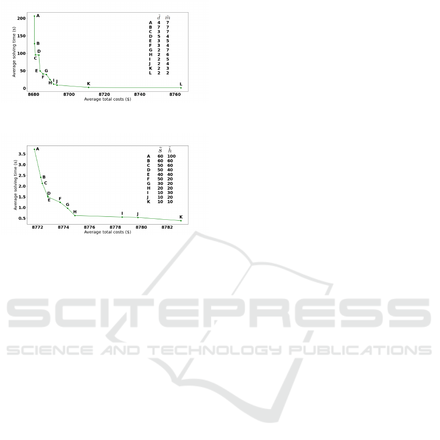
Figure 1: Resulting Pareto front for the MIP approach on

the training set with tested hyperparameter combinations.

Figure 2: Resulting Pareto front for the DP approach on the

training set with tested hyperparameter combinations.

as well as costs and consumed quantities of each en-

ergy source. The solving time is computed over 30

runs with a 95% conﬁdence interval. We also dis-

tinguish the solving time of the algorithms (Internal)

from the calls to OpenAP (External) since OpenAP

can take a considerable amount of time to compute its

predictions. The fuel costs do not vary in instance TB,

thus the DP+GD method is omitted due to returning

the same solution as DP.

For the solving time, we observe that MIP has on

average a statistically lower total solving time com-

pared to DP and DP+GD. However, DP and DP+GD

have on average a statistically lower internal solving

time than MIP, meaning that most of the time of these

methods is inside external calls to OpenAP. This ex-

ternal time could a priori be reduced by using caching

techniques or different external models. Thus, we can

conclude that DP and DP+GD have globally a smaller

solving time than MIP.

For the costs, we observe that MIP has the small-

est total cost for all instances. Compared to DP, its

total cost is on average 376.82$ (4.31%) smaller, with

a difference going from 53.94$ (1.17%) to as much

as 692.44$ (7.39%). Compared to DP+GD, its to-

tal cost is on average 144.96$ (1.67%) smaller, with

a difference going from 17.80$ (0.28%) to 502.78$

(5.37%). Compared to the heuristics, MIP is on

average 695.05$ (8.75%) smaller than MB-H and

1135.91$ (14.68%)) smaller than FF-H, with a max-

imum reduction of 1443.75$ (22.62%). For all in-

stances, the cost reduction mainly comes from a

greater electricity usage, with an increased electric-

ity consumption and costs, to allow for a smaller

fuel consumption. We also observe that, for most in-

stances, MIP has larger schedule costs, implying that

its higher electricity usage also comes from taking ad-

vantage of the soft schedule. Notably, it tends to ar-

rive earlier at terminals in order to increase its avail-

able charging time.

The MIP method always has the greatest electric-

ity consumption of all the methods. This allows to

reduce the fuel consumption on average by 119.2 L

(1.79%) in comparison with DP+GD, with a reduction

of up to 680.4 L (11.79%) compared to FF-H which

focuses on using fuel as much as possible. Further-

more, DP has a smaller fuel consumption than MIP

for two instances: OT (88.6 L, 1.58%) and ST (122.4

L, 1.39%). Thus, the optimal solution minimizing to-

tal costs is, for some instances, not always the solution

that minimizes the fuel consumption.

6.5 Scalability Analysis

We tested the scalability of the proposed approaches

by conducting an experimentation where the size of

instances was artiﬁcially increased to a given number

of terminals. For any instance, we can increase its

size by appending at its end the same ﬂights again up

to any terminal in the instance. For example, instance

PN with 4 terminals could be increased to 8 terminals

by doing all the ﬂights in its route twice. Thus, for

all instances in the test set, we increased their size to

10, 15, 20, and 25 terminals and computed the av-

erage total solving time of each method with a com-

putation timeout of 54 hours. Figure 3 presents the

results as a semi-log plot of the average total solving

time of each method given the number of terminals.

We observe that MIP can only solve instances of up

to 15 terminals in less than 20 minutes. In contrast,

DP and DP+GD clearly show a smaller increase in

solving time as the number of terminals increase and

thus scale better than the MIP approach. DP shows a

linear trend with a R

of 0.99. This is expected since

(Desch

enes et al., 2023) show that its time complex-

ity is pseudo-linear with the number of nodes in the

instance, which is directly proportional to the number

of terminals. However, DP+GD shows an exponen-

tial trend with a R

of 0.99. This can be explained

by the fact that the gradient descent post-treatment

can take an exponential time to converge. Similarly,

MIP clearly shows an exponential trend with a R

0.95 with an average total solving time higher than

DP and DP+GD for 15 terminals and above. The MIP

method on TB with 25 terminals reached the computa-

tion timeout of 54 hours with a relative gap of 0.14%.

ICORES 2025 - 14th International Conference on Operations Research and Enterprise Systems

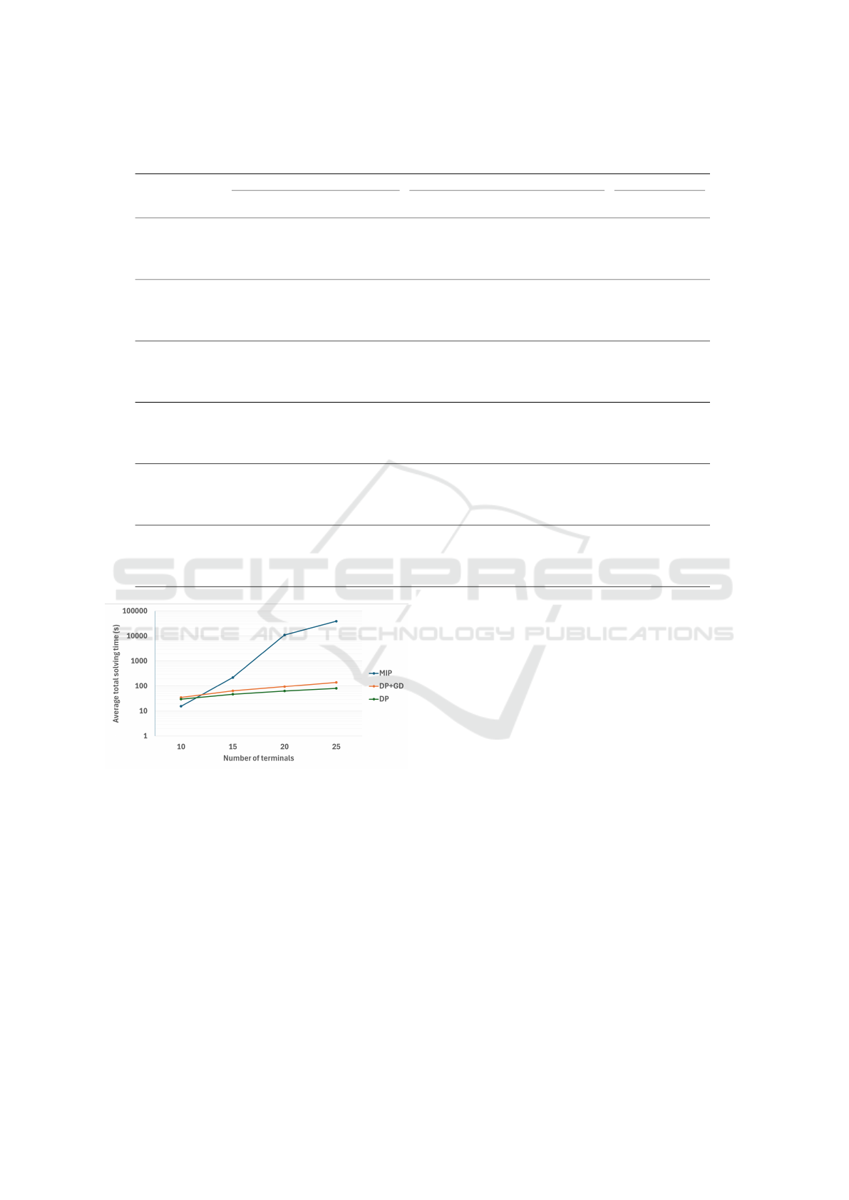
Table 5: Solving time of each instance in seconds — distinguished between internal (algorithms) and external (OpenAP) time

— as well as costs and consumed quantities of energy. Results reported for the DP, DP+GD, MIP, FF-H, and MB-H methods.

Instance Method

Solving time (s) Costs ($) Consumption

Internal External Total Fuel Electricity Schedule Total

Fuel

(L)

Electricity

(kWh)

DP 0.63 ± 0.06 12.02 ± 0.48 12.65 ± 0.53 4517.18 142.25 0.77 4660.20 3117.2 683.1

DP+GD - - - - - - - - -

MIP 4.42 ± 0.38 0.04 ± 0.00 4.46 ± 0.38 4448.19 152.85 5.21 4606.25 3066.8 732.2

FF-H 0.00 ± 0.00 0.09 ± 0.01 0.08 ± 0.00 5421.53 0.78 0.77 5422.08 3739.8 3.4

MB-H 0.02 ± 0.01 0.67 ± 0.03 0.69 ± 0.03 4817.62 124.51 0.77 4942.90 3319.5 572.2

DP 0.66 ± 0.10 13.68 ± 0.59 14.34 ± 0.67 6577.00 94.67 3.22 6674.89 5533.3 1070.4

DP+GD 0.82 ± 0.07 16.36 ± 0.55 17.18 ± 0.59 6301.30 94.66 3.22 6399.18 5648.1 1070.4

MIP 1.68 ± 0.32 0.03 ± 0.00 1.71 ± 0.32 6280.22 96.88 4.28 6381.38 5621.9 1096.7

FF-H 0.00 ± 0.00 0.09 ± 0.01 0.09 ± 0.01 7821.26 0.65 3.22 7825.14 6540.4 6.8

MB-H 0.03 ± 0.01 0.80 ± 0.03 0.83 ± 0.03 7277.74 84.47 3.22 7365.44 5853.0 937.7

DP 0.72 ± 0.11 15.31 ± 1.45 16.04 ± 1.54 7994.60 90.35 0.92 8085.87 6389.5 908.1

DP+GD 1.00 ± 0.15 18.19 ± 1.79 19.19 ± 1.90 7795.95 89.54 0.92 7886.41 6428.2 902.4

MIP 6.85 ± 0.26 0.04 ± 0.00 6.89 ± 0.26 7643.36 105.16 11.95 7760.47 6296.5 1039.1

FF-H 0.00 ± 0.00 0.10 ± 0.01 0.10 ± 0.01 9011.19 0.52 0.92 9012.63 7193.5 4.7

MB-H 0.04 ± 0.01 1.16 ± 0.03 1.20 ± 0.03 8304.79 73.99 0.92 8379.70 6636.8 723.6

DP 0.87 ± 0.08 18.00 ± 1.27 18.87 ± 1.34 10 558.1 50.86 0.52 10 609.48 8669.0 488.9

DP+GD 0.96 ± 0.10 19.81 ± 1.62 20.77 ± 1.71 9992.87 50.85 7.49 10 051.21 8867.4 488.8

MIP 4.66 ± 0.24 0.05 ± 0.00 4.72 ± 0.24 9887.23 54.24 2.28 9943.75 8791.4 526.4

FF-H 0.00 ± 0.00 0.12 ± 0.01 0.11 ± 0.00 11 129.70 0.60 0.52 11 120.83 9133.1 5.6

MB-H 0.05 ± 0.02 1.92 ± 0.03 1.97 ± 0.03 10 740.08 39.77 0.52 10 780.37 8823.9 366.1

DP 1.10 ± 0.08 23.10 ± 1.00 24.20 ± 1.06 13 032.49 79.02 0.61 13 112.13 10 612.5 670.2

DP+GD 1.17 ± 0.09 24.21 ± 0.67 25.38 ± 0.73 12 864.52 79.02 0.54 12 944.08 10 676.9 670.1

MIP 6.02 ± 0.23 0.08 ± 0.02 6.10 ± 0.23 12 786.33 87.03 8.88 12 882.24 10 606.7 732.5

FF-H 0.00 ± 0.00 0.17 ± 0.01 0.17 ± 0.01 13 892.69 0.46 0.61 13 894.76 11 303.8 3.6

MB-H 0.09 ± 0.02 3.13 ± 0.06 3.22 ± 0.05 13 334.31 68.58 0.61 13 403.79 10 856.6 544.7

DP 0.86 ± 0.06 17.49 ± 0.68 18.35 ± 0.71 10 013.70 29.87 20.15 10 063.71 7398.5 336.1

DP+GD 0.98 ± 0.08 19.65 ± 0.46 20.64 ± 0.53 9795.97 29.86 48.22 9874.05 7550.8 336.1

MIP 2.22 ± 0.37 0.05 ± 0.00 2.26 ± 0.36 9286.90 68.34 16.03 9371.27 7189.0 686.8

FF-H 0.00 ± 0.00 0.11 ± 0.02 0.10 ± 0.02 10 470.68 0.30 15.45 10 486.44 7744.1 2.7

MB-H 0.04 ± 0.02 1.75 ± 0.27 1.79 ± 0.26 10 204.31 23.71 15.45 10 243.48 7532.0 260.7

Figure 3: Semi-log plot of the average total solving time

by DP, DP+GD, and MIP with respect to the number of

terminals in the instances.

6.6 Discussion

Results from Section 6 demonstrate that the MIP ap-

proach always yields better solutions than the DP ap-

proach, but that the latter has a smaller internal solv-

ing time. This is expected, since the MIP is the only

method capable of leveraging the soft schedule. Un-

like other methods, which strictly adhere to the sched-

ule and sometimes result in smaller charging win-

dows, the MIP can choose to arrive earlier at a ter-

minal, thus extending the available charging window.

While this strategy incurs a cost for deviating from

the schedule, it allows for a longer charging duration

(which also incurs an additional cost), ultimately in-

creasing the available electrical energy for the sub-

sequent ﬂight. This increase in electricity reduces

the fuel required for the next ﬂight, thereby lower-

ing fuel costs. The primary advantage of the MIP

lies in its ability to identify scenarios where the re-

duction in fuel costs outweighs the combined costs

associated with deviating from the schedule and in-

creased electricity consumption. On the other hand,

considering the soft schedule and all its different sce-

narios can cause higher solving time, thus explaining

why the MIP has higher solving time than the other

approaches.

Thus, each approach has its beneﬁts and draw-

backs. With an average reduction of 145$ using the

MIP method compared to the DP+GD method, air-

craft operators in a real-life setting should evaluate if

this cost reduction is proﬁtable enough, notably when

taking into account the costs of hosting such an ap-

proach (e.g., solver license costs and infrastructure).

On the other hand, the DP approach has the advantage

of having fewer hardware limitations (e.g., memory

usage). Moreover, the MIP approach does not scale

well on larger instances and could take days to solve,

while DP could take less than 10 minutes.

A Mixed-Integer Programming Approach for an Extended Fixed Route Hybrid Electric Aircraft Charging Problem

On realistic instances, the MIP approach ﬁnds the

optimal solution in less than 7 seconds, which makes

it an interesting choice for a real-life planning con-

text. In addition, it is easier to improve and maintain,

while it can take into consideration a wider range of

constraints. It is thus easier to build on this approach

to solve variants of the FRHACP and its extension.

The MIP approach is also guaranteed to return an op-

timal solution (given its approximations), while the

DP methods are only heuristics for this problem. We

believe that greater variance in fuel, electricity and

schedule costs could lead to greater cost differences

between the approaches.

7 CONCLUSION

In this paper, we introduced an extended version

of the FRHACP incorporating additional constraints

and soft schedule requirements. To solve both the

FRHACP and its extension, we proposed a MIP ap-

proach. Through a comparative analysis involving a

benchmark of 10 realistic instances, we compared the

MIP approach against an updated DP approach ini-

tially introduced in previous work for the FRHACP.

Our ﬁndings consistently demonstrated that the MIP

approach yields superior solutions than DP, both

with and without gradient descent post-treatment,

achieving average cost reductions of 145$ (1.7%) and

377$ (4.3%), respectively. However, we showed that

it also requires a longer solving time compared to

the DP approach. Furthermore, our analysis revealed

that the MIP approach exhibits signiﬁcantly lower

scalability than its counterpart, thus each method has

its advantages and limitations. Directions for future

work include performing a sensitivity analysis on the

impact of the different parameters, as well as consid-

ering a variable aircraft speed.

ACKNOWLEDGMENTS

This work received ﬁnancial support from the Con-

sortium for Research and Innovation in Aerospace in

Quebec (CRIAQ) and the Mitacs Accelerate program.

The authors would like to thank the many members of

the Thales project team for their feedback on the prob-

lem deﬁnition and for the prototype implementation,

especially Vanessa Simard for her contribution on the

benchmark creation methodology.

REFERENCES

Ansarey, M., Shariat Panahi, M., Ziarati, H., and Mahjoob,

M. (2014). Optimal energy management in a

dual-storage fuel-cell hybrid vehicle using multi-

dimensional dynamic programming. Journal of Power

Sources, 250:359–371.

Ansell, P. J. and Haran, K. S. (2020). Electriﬁed airplanes:

A path to zero-emission air travel. IEEE Electriﬁca-

tion Magazine, 8(2):18–26.

De Cauwer, C., Verbeke, W., Coosemans, T., Faid, S., and

Van Mierlo, J. (2017). A data-driven method for

energy consumption prediction and energy-efﬁcient

routing of electric vehicles in real-world conditions.

Energies, 10(5):608.

Desch

enes, A., Boudreault, R., Simard, V., Gaudreault, J.,

and Quimper, C.-G. (2023). Dynamic programming

for the ﬁxed route hybrid electric aircraft charging

problem. In Wu, W. and Guo, J., editors, Combina-

torial Optimization and Applications, Lecture Notes

in Computer Science, pages 354–365, Cham. Springer

Nature Switzerland.

Desch

enes, A., Gaudreault, J., and Quimper, C.-G. (2022).

Predicting real life electric vehicle fast charging ses-

sion duration using neural networks. In 2022 IEEE In-

telligent Vehicles Symposium (IV), pages 1327–1332.

Desch

enes, A., Gaudreault, J., Rioux-Paradis, K., and Red-

mont, C. (2020a). Predicting electric vehicle con-

sumption: A hybrid physical-empirical model. World

Electric Vehicle Journal, 11(1):2.

Desch

enes, A., Gaudreault, J., Vignault, L.-P., Bernard, F.,

and Quimper, C.-G. (2020b). The ﬁxed route electric

vehicle charging problem with nonlinear energy man-

agement and variable vehicle speed. In 2020 IEEE

International Conference on Systems, Man, and Cy-

bernetics (SMC), pages 1451–1458.

Ehrgott, M. and Tenfelde-Podehl, D. (2003). Computation

of ideal and Nadir values and implications for their use

in MCDM methods. European Journal of Operational

Research, 151(1):119–139.

Lin, J., Zhou, W., and Wolfson, O. (2016). Electric vehicle

routing problem. Transportation Research Procedia,

12:508–521.

Mancini, S. (2017). The hybrid vehicle routing problem.

Transportation Research Part C: Emerging Technolo-

gies, 78:1–12.

Misener, R. and Floudas, C. A. (2010). Piecewise-

linear approximations of multidimensional functions.

Journal of Optimization Theory and Applications,

145(1):120–147.

Montoya, A., Gu

eret, C., Mendoza, J. E., and Villegas, J. G.

(2017). The electric vehicle routing problem with

nonlinear charging function. Transportation Research

Part B: Methodological, 103:87–110.

Nethercote, N., Stuckey, P. J., Becket, R., Brand, S., Duck,

G. J., and Tack, G. (2007). MiniZinc: Towards a stan-

dard CP modelling language. In Bessi

ere, C., edi-

tor, Principles and Practice of Constraint Program-

ming – CP 2007, Lecture Notes in Computer Science,

ICORES 2025 - 14th International Conference on Operations Research and Enterprise Systems

pages 529–543, Berlin, Heidelberg. Springer. Web-

site: https://www.minizinc.org/.

Pinto Leite, J. P. S. and Voskuijl, M. (2020). Optimal energy

management for hybrid-electric aircraft. Aircraft En-

gineering and Aerospace Technology, 92(6):851–861.

Seyﬁ, M., Alinaghian, M., Ghorbani, E., C¸ atay, B., and Sab-

bagh, M. (2022). Multi-mode hybrid electric vehicle

routing problem. Transportation Research Part E: Lo-

gistics and Transportation Review, 166:102882.

Sun, J., Hoekstra, J. M., and Ellerbroek, J. (2020). Ope-

nAP: An open-source aircraft performance model for

air transportation studies and simulations. Aerospace,

7(8):104.

Yu, V. F., Redi, A. A. N. P., Hidayat, Y. A., and Wibowo,

O. J. (2017). A simulated annealing heuristic for the

hybrid vehicle routing problem. Applied Soft Comput-

ing, 53:119–132.

Zhen, L., Xu, Z., Ma, C., and Xiao, L. (2020). Hy-

brid electric vehicle routing problem with mode selec-

tion. International Journal of Production Research,

58(2):562–576.

A Mixed-Integer Programming Approach for an Extended Fixed Route Hybrid Electric Aircraft Charging Problem