Impact of Balancing and Regularization on the Semantic Segmentation

of Gleason Patterns

Eduardo Henrique S. Paraíso

1 a

and Alexei M. C. Machado

1,2 b

PPGInf - Graduate Program on Informatics, Pontiﬁcal Catholic University of Minas Gerais,

Dom José Gaspar 500, Belo Horizonte, Brazil

Department of Anatomy and Imaging, Universidade Federal de Minas Gerais,

Alfredo Balena 190, Belo Horizonte, Brazil

Keywords:

Image Segmentation, Deep Learning, Class Balancing, Regularization, Prostate Cancer.

Abstract:

This study investigates the impact of class balancing and regularization on improving the diagnostic agreement

in prostate histological images. The U-Net models applied to the Prostate Cancer Grade Assessment dataset

reveal that class balancing combined with traditional loss functions contributes to an increase of up to 6

percentage points in image agreement. Combining balancing and Focal Loss can increase image classiﬁcation

agreement by an average of 13 percentage points compared to using an imbalanced dataset with traditional

loss functions. Notably, distinguishing between Gleason patterns 3 and 4 in medical image analysis is crucial,

as this distinction not only directly inﬂuences clinical decisions and the prognosis of prostate cancer patients

but also emphasizes the need for careful interpretation of the data.

1 INTRODUCTION

Prostate adenocarcinoma (PA) is the most common

cancer among men worldwide, accounting for 10.2%

of male cancer diagnoses in Brazil, with 72,000 new

cases projected for 2023–2025 (INCA, 2023). Di-

agnosis relies on prostate biopsy and the Gleason

grading system (Gleason and Mellinger, 1974), which

evaluates tumor cell differentiation on a scale of 1 to

5 (Figure 1), with patterns 3 and 4 indicating moder-

ate and high malignancy. However, distinguishing be-

tween these patterns is challenging due to subtle mor-

phological differences, leading to diagnostic discrep-

ancies of 30–53% (Ozkan et al., 2016). These inac-

curacies affect treatment decisions, such as prostate-

ctomy, which can cause severe side effects. Accurate

differentiation is essential to avoid overtreatment and

improve patient outcomes.

Artiﬁcial intelligence (AI), especially deep learn-

ing (DL), is increasingly used in medical decision-

making, providing diagnostic results comparable to

specialists (Raciti et al., 2020). Convolutional Neural

Networks (CNNs), including U-Net-based architec-

tures like Residual U-Net (Kalapahar et al., 2020) and

Residual Attention U-Net (Damkliang et al., 2023),

https://orcid.org/0009-0004-9236-8300

https://orcid.org/0000-0001-8077-3377

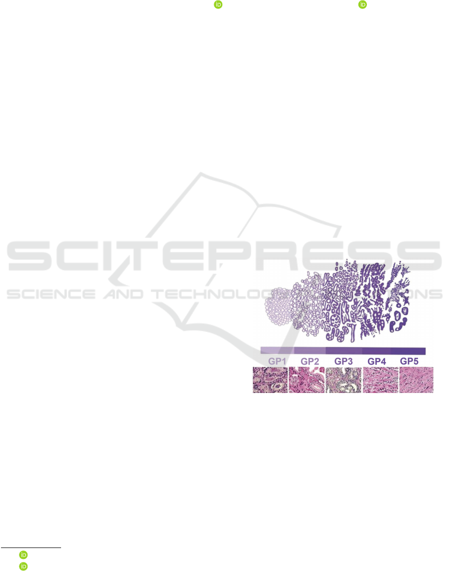
Figure 1: Gleason Pattern scale: GP1 - Regular, uniform,

and small cells; GP2 - Uniform cells, loosely grouped, and

irregular borders; GP3 - Very small, uniform cells, angu-

lar or elongated; GP4 - Many cells fused into large amor-

phous masses; GP5 - Large masses with invasion of neigh-

boring organs and tissues, minimal glandular differentia-

tion. Adapted from: University of Pittsburgh Medical Cen-

ter (UPMC) Cancer Centers, Pittsburgh, PA, USA.

are commonly applied for Gleason pattern (GP) seg-

mentation. However, distinguishing between GP 3

and 4 remains challenging due to low agreement in

results, limiting DL’s clinical use. Additionally, class

imbalance in training data introduces bias, reduc-

ing the models’ effectiveness in detecting minority

classes (Dablain et al., 2024).

382

Paraíso, E. H. S. and Machado, A. M. C.

Impact of Balancing and Regularization on the Semantic Segmentation of Gleason Patterns.

DOI: 10.5220/0013105500003911

Paper published under CC license (CC BY-NC-ND 4.0)

In Proceedings of the 18th International Joint Conference on Biomedical Engineering Systems and Technologies (BIOSTEC 2025) - Volume 2: HEALTHINF, pages 382-389

ISBN: 978-989-758-731-3; ISSN: 2184-4305

This article

investigates, through an ablative

study (Meyes et al., 2019), the impact of class bal-

ancing in DL models applied to the semantic segmen-

tation of histological images of the prostate and the

effect of regularization for the prevention of overﬁt-

ting, when applying a loss function designed to handle

class imbalance in classiﬁcation problems. The study

is speciﬁcally directed to the evaluation of the U-Net

models. Ultimately, we aim to increase the accuracy

and agreement metrics of GP 3 and 4 to increase the

patient’s chances of cure and treatment effectiveness.

This structure: Section 2 reviews studies on se-

mantic segmentation in prostate image datasets, high-

lighting the use and importance of balancing in these

datasets. Section 3 explores the fundamental concepts

necessary for a deeper understanding of this work.

Section 4 presents the methodology adopted in this

study. Section 5 explores the results achieved during

the experiments. Finally, Section 6 offers the conclud-

ing remarks and outlines future work.

2 RELATED WORKS

Bulten et al. (2022) conducted a comparative analysis

between CNNs and pathologists using the Quadratic

Weighted Kappa (QWK) metric, showing that CNNs

often outperformed pathologists in accuracy, sensitiv-

ity, and speciﬁcity. However, their study did not fo-

cus on CNN performance for Gleason patterns 3 and

4. Similarly, Silva-Rodríguez et al. (2020) achieved a

QWK of 77% when evaluating prostate cancer diag-

nosis on the SICAPv2 dataset, which shares charac-

teristics with the dataset used in this work.

Ikromjanov et al. (2022) achieved F1-scores of

78% and 67% for classifying GP3 and GP4 on the

Prostate Cancer Grade Assessment (PANDA) dataset,

using 256×256 pixel patches without reporting addi-

tional preprocessing techniques. This suggests that

further exploration of preprocessing methods could

lead to improved and more competitive results.

Guerrero et al. (2024) explored data augmentation

techniques to address data imbalance in histopatho-

logical datasets, focusing on classiﬁer-level and data-

level solutions to improve CNN performance. Anal-

ogously, Falahkheirkhah et al. (2023) investigated the

use of deepfake technologies, particularly Generative

Adversarial Networks (GANs), to synthesize realistic

histological images for medical image analysis, clas-

siﬁcation tasks, and data augmentation.

The repository of the work can be accessed at https:

//www.drive.google.com/drive/folders/1k9AEAkq9X\\4B9

QcjOziEq2Bjw6xwKfNUD

Hancer et al. (2023) focused on addressing the

class imbalance in nucleus segmentation in hema-

toxylin and eosin (H&E) stained histopathological

images using the U-Net architecture. Similarly,

(Haghofer et al., 2023) and Chen (2023) demonstrated

the high performance of U-Net and its variants in

medical image segmentation tasks, including cell and

nucleus segmentation, emphasizing its effectiveness

in histological image analysis.

The study discussed in this work is speciﬁcally re-

lated to two previous research efforts: Guerrero et al.

(2024), which uses a Mask Region-Based Convolu-

tional Neural Networks (R-CNN) model enhanced by

a modiﬁed copy-paste data augmentation technique to

improve the training process and help class balancing,

and Chen (2023), which employs a U-Net model for

prostate image analysis. This study distinguishes it-

self by using an ablative methodology to analyze the

impact of class balancing and regularization, enhanc-

ing understanding of their roles in semantic tissue seg-

mentation and their effect on classifying Gleason pat-

terns 3 and 4.

3 BACKGROUND

Selecting suitable metrics is vital for accurately as-

sessing a model’s performance in the given context.

The loss functions play a key role in guiding training,

enabling the model to distinguish between patterns ef-

fectively. This ensures precise and clinically mean-

ingful segmentation of Gleason patterns, leading to

improved diagnosis and more appropriate treatments.

3.1 Segmentation Models

The U-Net architecture introduced by Ronneberger

et al. (2015)is a leading semantic segmentation model

known for its efﬁciency and robust performance. De-

signed for biomedical tasks, it uses a contracting path

to capture spatial context and an expansive path for

precise localization. Its U-shaped structure enables

accurate segmentation even with limited data, making

it widely used in medical and computer vision appli-

cations.

The loss function is pivotal in optimizing semantic

segmentation models, ensuring the network’s output

is appropriately compared to ground truth labels. The

most common loss function combines cross-entropy

(CEL), which evaluates the similarity between the

predicted segmented mask and the ground truth mask,

with regularization terms to prevent overﬁtting. The

CEL function is deﬁned as:

CEL = −

∑

i=1

log( ˆy

), (1)

Impact of Balancing and Regularization on the Semantic Segmentation of Gleason Patterns

383

where N is the total number of classes, y

represents a

vector with the true class, and ˆy

represents the prob-

ability of the predicted class. This encourages precise

learning of the discriminative characteristics of each

class (R ˛aczkowska et al., 2019).

Focal loss (FL), proposed by Lin et al. (2018),

was explored as an alternative to cross entropy (CEL)

to handle class imbalance in classiﬁcation problems.

It adds a modulating term, (1 − ˆy

)

, to CEL, where

γ > 0 reduces the loss for well-classiﬁed examples.

An optional balancing factor, α

, can also be used to

address class imbalances:

FL = −α

(1− ˆy

)

log ˆy

. (2)

This approach is beneﬁcial in datasets with minority

classes, improving network performance as demon-

strated by Nguyen et al. (2024).

3.2 Metrics

The performance of the models were assessed based

on a set of well-known metrics:

1. Sensitivity (recall) shows the proportion of true

positives relative to total positive cases, including

false negatives (FN) (Powers, 2015).

2. Speciﬁcity is the proportion of genuinely nega-

tive observations in the dataset (Monaghan et al.,

2021). This indicates the model’s ability to avoid

false positives.

3. The F1-Score is a key metric for evaluating classi-

ﬁcation models, particularly in cases of class im-

balance. It is the harmonic mean of precision and

recall. It is useful when a balance between the two

is needed, especially when one type of error (false

positives or false negatives) has a greater impact

(Hicks et al., 2022).

4. Quadratic Weighted Kappa (QWK) is a statisti-

cal measure that assesses agreement among raters

when discrepancies between their classiﬁcations

have different weights, considering the distance

between categories. The difference between

classes is weighted using a quadratic factor. The

weight for the cell in row i and column j of the

matrix is given by

W (i, j) = (i − j)

/(N − 1)

, (3)

where N is the total number of categories.

The QWK is calculated by comparing the

weighted confusion matrix with the weighted ex-

pectation matrix:

QWK = 1 −

∑

W (i, j)O(i, j)

∑

W (i, j)E(i, j)

, (4)

where O

i j

is the observed frequency of agreement

among raters in the category and E

i j

is the ex-

pected frequency of agreement in the category.

The quadratic weighting assigns larger weights to

more distant discrepancies on the ordinal scale.

By applying these weights, QWK gives more

importance to severe disagreements, resulting in

smaller values than simple Kappa, thus, QWK is

useful for assessing the reproducibility of diag-

nostic methods with ordinal variables (Silva et al.,

2016). However, QWK evaluates overall agree-

ment across classiﬁcations. It provides an aggre-

gate view, reﬂecting the general level of agree-

ment across all classes.

4 MATERIALS AND METHODS

The PANDA dataset

was developed jointly by the

computational pathology group at Radboud Univer-

sity Medical Center (RUMC) and the Department

of Medical Epidemiology and Biostatistics at the

Karolinska Institute (DEMBIK) (Bulten et al., 2022).

The dataset comes from needle core biopsies per-

formed between 2012 and 2017. Due to the subjec-

tive nature of GPs, classiﬁcation divergences arise, as

noted by Corte (2023), who highlights that the im-

age labels contain signiﬁcant noise from inconclu-

sive records, annotation errors, diagnostic inaccura-

cies, and pathologist discrepancies.

The dataset comprises 10,616 high-resolution im-

ages stained with H&E pigments and stored in TIFF

(Tagged Image File Format) format. These images

were obtained through optical microscopy and digi-

tized to create high-resolution digital versions with an

objective lens magniﬁcation of 20x. An essential fea-

ture of WSIs is their ability to provide multiple mag-

niﬁcation levels (see Figure 2a), where the original

image is subdivided into various resolutions.

The specimens provided by DEMBIK were la-

beled by regions (see Figure 2b) into background, be-

nign tissue, and cancerous tissue. In contrast, RUMK

performed a more detailed classiﬁcation (see Figure

2b) by individually labeling the cytoarchitecture into

background, stroma, GP2, GP3, GP4, and GP5.

In order to investigate the impact of balancing and

regularization through the ablative approach, the U-

Net models were trained using combinations of im-

balanced and balanced image datasets, along with var-

ious pixel normalization and loss functions, resulting

in a total of 24 trained models. All models were

https://www.kaggle.com/competitions/prostate-cance

r-grade-assessment

HEALTHINF 2025 - 18th International Conference on Health Informatics

384

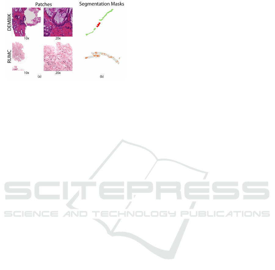
Figure 2: (a) Multiple levels of magniﬁcation provided by

the pyramidal structure of a WSI. (b) Full segmentation

mask of a WSI.

trained using 10-fold cross-validation (using a T4

GPU and 28GB of RAM), and a 95% conﬁdence in-

terval was calculated. The ablative approach is help-

ful for better understanding how different components

of the training process affect the model’s ﬁnal perfor-

mance. In this case, ablating data balancing allows for

evaluating how the imbalance between data classes

inﬂuences segmentation metrics, especially between

GP3 and GP4.

4.1 Image Selection and Preprocessing

A total of 5,160 images from the PANDA dataset orig-

inating from RUMC were selected due to their in-

dividualized glandular annotations (Figure 3a). For

training, 330 WSIs were selected, and 80 WSIs for

testing through stratiﬁed random sampling (Figure

3b). Stratiﬁcation was based on the Gleason Score,

a histological classiﬁcation system consisting of two

numerical scores ranging from 3 to 5, representing the

two predominant tumor patterns in the tissue. Adopt-

ing the ablative approach involves a wide range of

combinations; thus, time constraints and hardware

limitations justiﬁed the design of this investigation.

4.2 Patch Generation

The use of patches is crucial for training models

on histological images, as it allows for diversiﬁca-

tion and captures localized details, improving the

model’s ability to recognize intricate features and nu-

ances (Dablain et al., 2024).

During patch generation, the alpha channel was

excluded because transparency is irrelevant for seg-

mentation tasks Alsayat et al. (2023), while the blue

and green channels, from masks, were omitted as

pixel classiﬁcation data is stored only in the red chan-

nel. Patches were created (Figure. 3c) with dimen-

sions of 224×224×3 for images and 224×224×1 for

masks. This size balances computational efﬁciency

with deep learning capabilities for high-dimensional

data (Ciga et al., 2021) and ensures compatibility with

widely used architectures, such as those trained on

ImageNet (Russakovsky and et al., 2015).

A sliding window approach was implemented

with a 10% overlap of the patch size, allowing for the

generation of patches with overlapping boundaries.

Among the generated patches, selecting images with

the highest representativeness was based on minimiz-

ing the pixels labeled as background. Patches with

a background proportion exceeding 10% of the to-

tal image area were excluded from the dataset, en-

suring a greater concentration of relevant pixels for

histopathological analysis.

After completing the described processing, 9,442

patches were obtained for the training set and 2,174

patches for the test set (Figure 3c).

Due to the images’ nature, the proportion of each

label was calculated, with the difference between the

majority class (stroma) and the minority class (GP3)

being 68%. Balancing was performed in four steps:

1. Images containing GP3 or GP4 were selected.

2. Patches with a composition of pixels classiﬁed as

stroma greater than 80% were removed.

3. Patches composed of more than 50% GP3 or GP4

were selected for artiﬁcial augmentation.

4. Transformations were applied to 512 GP3 and

937 GP4 patches, generating four new images per

original GP3 patch and one new image per origi-

nal GP4 patch.

The following transformations were used for the

data augmentation:

a. Random contrast and brightness;

b. Rotation, limited to 35º;

c. Horizontal and/or Vertical ﬂipping;

After the balancing step of the training set (see

Figure 5d), a ﬁnal set of 6,700 patches was obtained,

with a class imbalance difference between the major-

ity and minority class of less than 30% (Figure 4).

4.3 Normalization

Both balanced and imbalanced image sets were an-

alyzed without any initial normalization. Then, two

different normalization techniques were applied: nor-

malization by maximum pixel value and normaliza-

tion by mean and standard deviation of the training

set. Each of these created sets was used to train 24

distinct models, employing different loss functions as

depicted in Figure 5.

Impact of Balancing and Regularization on the Semantic Segmentation of Gleason Patterns

385

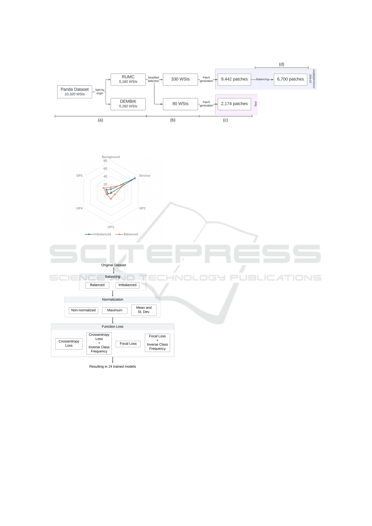
Figure 3: (a) Separation of the image set according to its source. (b) The training and testing sets are created through stratiﬁed

random selection from the RUMC dataset. (c) Selected set of patches with at least 90% relevant area for classiﬁcation. (d)

The ﬁnal set of patches resulted from class balancing.

Figure 4: Distribution of classes in the original dataset

(blue) and balanced dataset (orange).

Figure 5: The ablative scheme proposed in this study com-

prises 24 distinct models, each resulting from the combina-

tion of three different steps: balancing or not balancing the

dataset, using a speciﬁc type of pixel normalization, and ap-

plying a loss function during training.

4.4 Loss Function

In addition to Cross Entropy Loss, this study uti-

lized Focal Loss, designed to handle scenarios with

extreme class imbalances. Additionally, CEL and

FL variations were employed, incorporating weights

based on inverse class frequency. This adjust-

ment mitigates potential biases and facilitates equi-

table model learning, promoting better generalization

and performance, particularly for underrepresented

classes. All models were based on a standard U-Net

architecture, following the implementation by Ron-

neberger et al. (2015).

5 RESULTS AND DISCUSSION

The FL demonstrates superior stability in cross-

validation results compared to CE and a more con-

sistent and steady reduction in loss values. This high-

lights the regularization capability of FL in mitigat-

ing the disparity between the model’s predictions and

the true data labels throughout the training process,

as illustrated in Figure 6a and 6b, which compare the

performance of these functions on an imbalanced and

non-normalized dataset.

The simultaneous application of FL with the bal-

ancing of the image set (Figure 6c) leads to a reduc-

tion in the distance between the training and valida-

tion loss curves. In DL models, this approximation

indicates a generalization capability, implying better

adaptation of the model to training data and, in turn,

a greater ability to predict new datasets accurately.

Such models are less prone to overﬁtting, ensuring

greater reliability and robustness in real world.

The Table 1 demonstrates the ability of Focal Loss

to mitigate the impact of majority classes in the clas-

siﬁcation of GPs 3 and 4 within a highly imbalanced

dataset, resulting in better model performance in bal-

ancing sensitivity and speciﬁcity. This indicates the

regularization potential of FL through class balanc-

ing, supported by the increased stability observed in

Figure 6b. Focal Loss stands out in F1-score met-

rics, showing a slight advantage compared to other

loss functions. However, it is not possible to deter-

mine which normalization is superior, as the results

HEALTHINF 2025 - 18th International Conference on Health Informatics

386

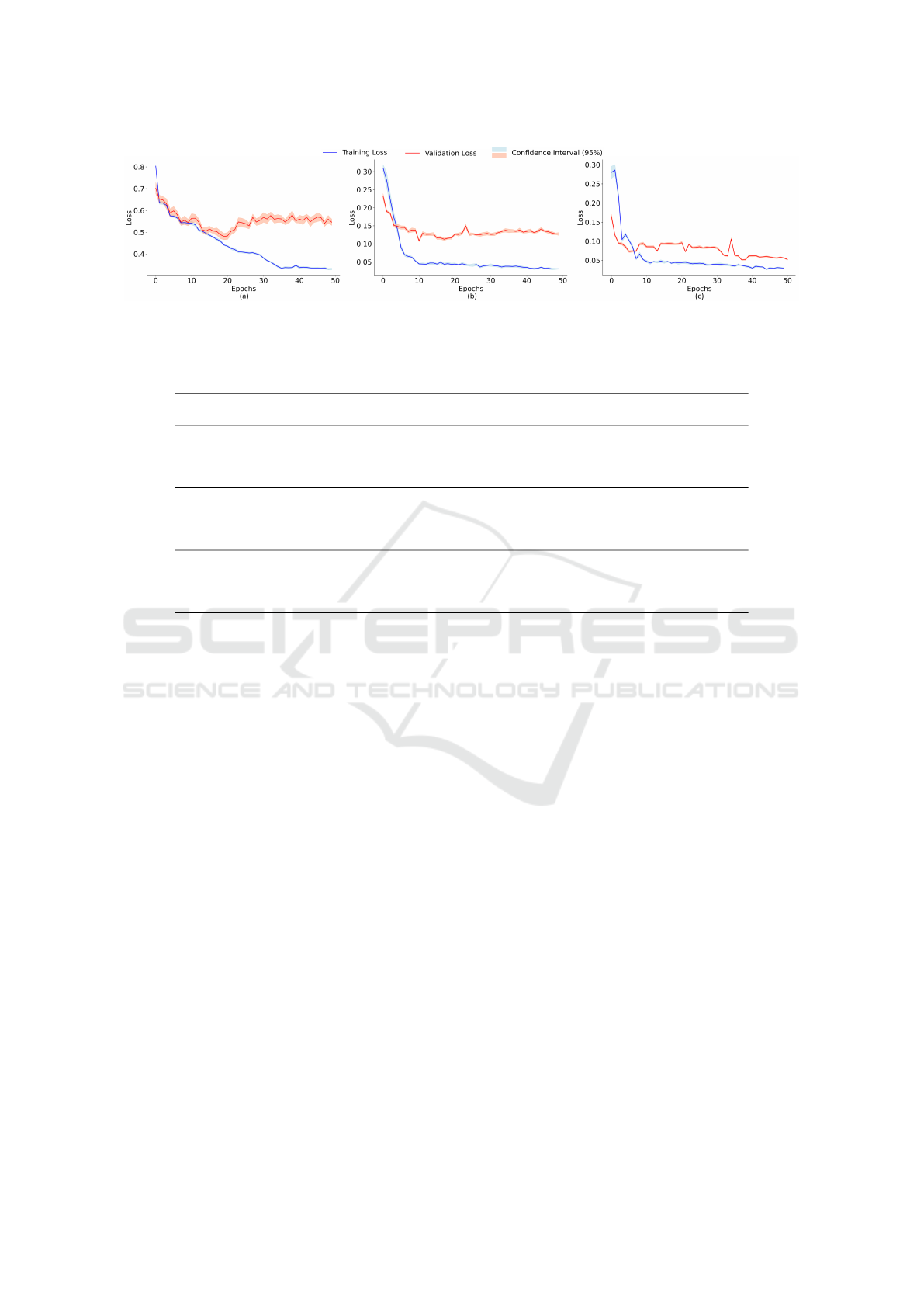
Figure 6: Loss functions resulting from 10-fold cross-validation for an imbalanced dataset using Cross-Entropy Loss (a), for

an imbalanced dataset using Focal Loss (b), and for a balanced dataset using Focal Loss (c) simultaneously.

Table 1: Results of 10-fold cross-validation and their respective 95% conﬁdence intervals for training on an imbalanced

dataset.

Normalization Loss

Gleason Pattern 3 Gleason Pattern 4

Sensitivity Speciﬁcity F1-Score Sensitivity Speciﬁcity F1-Score

Non-normalized

CEL 0.66 ± 0.02 0.97 ± 0.03 0.61 ± 0.02 0.37 ± 0.02 0.95 ± 0.01 0.46 ± 0.03

CEL+ICF 0.58 ± 0.06 0.82 ± 0.08 0.57 ± 0.04 0.30 ± 0.07 0.88 ± 0.02 0.35 ± 0.07

FL 0.72 ± 0.02 0.95 ± 0.01 0.66 ± 0.03 0.40 ± 0.01 0.97 ± 0.01 0.52 ± 0.02

FL+ICF 0.64 ± 0.04 0.90 ± 0.04 0.59 ± 0.03 0.34 ± 0.03 0.93 ± 0.03 0.40 ± 0.04

Maximum

CEL 0.73 ± 0.01 0.95 ± 0.02 0.63 ± 0.02 0.39 ± 0.02 0.96 ± 0.03 0.46 ± 0.01

CEL+ICF 0.57 ± 0.04 0.94 ± 0.03 0.52 ± 0.05 0.37 ± 0.02 0.91 ± 0.08 0.39 ± 0.02

FL 0.76 ± 0.03 0.96 ± 0.01 0.68 ± 0.01 0.41 ± 0.03 0.95 ± 0.02 0.50 ± 0.01

FL+ICF 0.65 ± 0.04 0.90 ± 0.02 0.58 ± 0.03 0.37 ± 0.03 0.88 ± 0.03 0.42 ± 0.03

Mean/St. Dev.

CEL 0.69 ± 0.02 0.95 ± 0.03 0.64 ± 0.02 0.34 ± 0.03 0.97 ± 0.02 0.47 ± 0.02

CEL+ICF 0.59 ± 0.04 0.90 ± 0.05 0.57 ± 0.02 0.40 ± 0.05 0.88 ± 0.09 0.40 ± 0.03

FL 0.78 ± 0.02 0.95 ± 0.03 0.69 ± 0.01 0.43 - 0.01 0.98 ± 0.02 0.53 ± 0.01

FL+ICF 0.63 ± 0.03 0.87 ± 0.02 0.59 ± 0.01 0.35 ± 0.03 0.91 ± 0.01 0.41 ± 0.02

of this metric overlap within the conﬁdence intervals.

The results highlighted in Table 2 highlight the

importance of dataset balancing, emphasizing the cru-

cial role of balance and regularization. The analysis

of the F1-score reveals a more signiﬁcant improve-

ment compared to models trained on an imbalanced

dataset, with approximately an increase of eight per-

centage points for GP3 and around 14 percentage

points for GP4, averaged across the three normaliza-

tions when trained using Focal Loss. However, de-

termining the best normalization is again not directly

possible, as the obtained values overlap when consid-

ering the conﬁdence intervals.

Analyzing the global image classiﬁcation results

through the QWK metric, it is observed that, on av-

erage, models trained on balanced image sets using

CEL achieved levels of agreement similar to those

obtained by models trained on imbalanced sets using

FL. Regardless of the normalization applied, FL could

return an average gain of 7 percentage points over

CEL for imbalanced datasets. When comparing this

metric for balanced datasets, FL showed an average

gain of 6 percentage points. Therefore, when compar-

ing the agreement between an imbalanced set trained

with CEL and a balanced set trained with FL, an ap-

proximate average gain of 13 percentage points is ob-

served. These results align with those obtained by

Silva-Rodríguez et al. (2020), despite being derived

from different image sets, both datasets share similar-

ities regarding objective lens magniﬁcation and his-

tochemical staining. Additionally, it is important to

note that in the competition organized on the Kaggle

platform, winning works achieved concordance val-

ues of approximately 90%. However, label denoising

techniques were employed to eliminate images with

discrepancies between the results obtained by CNNs

and segmentation masks. While effective in remov-

ing erroneously labeled images that hinder training,

this technique is also responsible for discarding im-

ages that are challenging to classify. Given the subjec-

tive nature and difﬁculty distinguishing between GP

3 and 4, such information may have been eliminated,

contributing to the high concordance values obtained.

Therefore, the results obtained in this study remain

competitive and highlight the importance of balanc-

ing and regularization in future research endeavors.

However, the application of a speciﬁc pixel nor-

malization technique did not signiﬁcantly improve

agreement (see Table 3), highlighting that normaliza-

tion’s impact varies by context. This underscores the

complexity of optimizing segmentation models, re-

quiring careful consideration of factors like data bal-

ancing and preprocessing techniques. While weight-

ing strategies can aid balancing, weights deﬁned by

Impact of Balancing and Regularization on the Semantic Segmentation of Gleason Patterns

387

Table 2: Results of 10-fold cross-validation and their respective 95% conﬁdence intervals for training on an balanced dataset.

Normalization Loss

Gleason Pattern 3 Gleason Pattern 4

Sensitivity Speciﬁcity F1-Score Sensitivity Speciﬁcity F1-Score

Non-normalized

CEL 0.77 ± 0.04 0.94 ± 0.02 0.71 ± 0.04 0.81 ± 0.02 0.95 ± 0.02 0.61 ± 0.04

CEL+ICF 0.65 ± 0.06 0.84 ± 0.3 0.60 ± 0.03 0.60 ± 0.05 0.80 ± 0.04 0.48 ± 0.09

FL 0.80 ± 0.01 0.94 ± 0.04 0.73 ± 0.02 0.80 ± 0.03 0.95 ± 0.04 0.66 ± 0.02

FL+ICF 0.72 ± 0.03 0.96 ± 0.02 0.66 ± 0.03 0.80 ± 0.02 0.90 ± 0.03 0.51 ± 0.06

Maximum

CEL 0.76 ± 0.01 0.95 ± 0.03 0.66 ± 0.03 0.82 ± 0.02 0.92 ± 0.01 0.60 ± 0.01

CEL+ICF 0.69 ± 0.03 0.85 ± 0.02 0.61 ± 0.05 0.60 ± 0.07 0.85 ± 0.02 0.58 ± 0.04

FL 0.78 ± 0.03 0.96 ± 0.02 0.75 ± 0.03 0.82 ± 0.03 0.96 ± 0.02 0.66 ± 0.03

FL+ICF 0.73 ± 0.02 0.93 ± 0.04 0.66 ± 0.04 0.73 ± 0.03 0.97 ± 0.01 0.60 ± 0.03

Mean/St. Dev.

CEL 0.78 ± 0.02 0.91 ± 0.02 0.73 ± 0.02 0.81 ± 0.04 0.95 ± 0.02 0.59 ± 0.02

CEL+ICF 0.70 ± 0.03 0.86 ± 0.01 0.59 ± 0.04 0.61 ± 0.02 0.84 ± 0.04 0.54 ± 0.05

FL 0.85 ± 0.02 0.97 ± 0.02 0.77 ± 0.01 0.81 ± 0.01 0.97 ± 0.01 0.65 ± 0.02

FL+ICF 0.75 ± 0.04 0.92 ± 0.03 0.66 ± 0.02 0.77 ± 0.01 0.96 ± 0.01 0.59 ± 0.04

Table 3: Results of 10-fold cross-validation and their respective 95% conﬁdence intervals for QWK metric for all models.

CEL CEL+ICF FL FL+ICF

Imbalanced

Non-normalized 0.57 ± 0.05 0.20 ± 0.14 0.65 ± 0.03 0.34 ± 0.04

Maximum 0.61 ± 0.03 0.23 ± 0.06 0.67 ± 0.02 0.40 ± 0.02

Mean/St. Dev 0.55 ± 0.02 0.21 ± 0.03 0.64 ± 0.02 0.51 ± 0.03

Balanced

Non-normalized 0.66 ± 0.02 0.25 ± 0.09 0.64 ± 0.06 0.60 ± 0.05

Maximum 0.65 ± 0.01 0.27 ± 0.07 0.70 ± 0.02 0.66 ± 0.02

Mean/St. Dev 0.62 ± 0.03 0.28 ± 0.02 0.73 ± 0.01 0.64 ± 0.02

ICF proved challenging for model convergence.

The use of inverse class frequency, combined

with the adopted loss functions, failed to improve

model performance and worsened the classiﬁcation

of GP3 and GP4, reducing agreement compared to

other methods. This may be due to overemphasis on

underrepresented classes, exacerbating class imbal-

ance and impairing generalization, especially when

the loss functions cannot handle such weighting ef-

fectively.

6 CONCLUSION

This study demonstrates that image balancing is cru-

cial for accurately diagnosing histological PA im-

ages and is an effective regularization strategy dur-

ing model training. It also emphasizes caution when

using moderating weights in loss functions, as im-

proper application can destabilize models or slow

convergence without improving accuracy. The study

achieved competitive results with minimal prepro-

cessing, highlighting the importance of balancing and

regularization techniques.

Efforts should focus on reducing dataset noise,

particularly in annotations, as it compromises pre-

diction quality. Addressing histological anomalies or

distortions from tissue preparation is also essential to

prevent analysis distortions. Implementing ensemble

techniques could improve the classiﬁcation of Glea-

son patterns 3 and 4, addressing a key challenge in the

ﬁeld. Additionally, exploring new architectures and

evaluating their speciﬁc behaviors is crucial, given the

limited research on this topic. These strategies could

signiﬁcantly enhance the understanding and analysis

of prostate adenocarcinoma.

ACKNOWLEDGMENTS

The authors thank the Pontifícia Universidade

Católica de Minas Gerais – PUC-Minas and

Coordenação de Aperfeiçoamento de Pessoal

de Nível Superior - CAPES - (Grant PROAP

88887.842889/2023-00 - PUC/MG, Grant PDPG

88887.708960/2022-00 - PUC/MG - INFOR-

MÁTICA and Finance Code 001). Conselho Nacional

de Desenvolvimento Cientíﬁco e Tecnológico do

Brasil (CNPq – Código:311573/2022-3). Scholarship

FAPEMIG/CNPq - Brazil (Grant BPQ-06556-24).

Grant FAPEMIG - Brazil APQ-02753-24.

REFERENCES

Alsayat, A., Elmezain, M., Alanazi, S., Alruily, M.,

Mostafa, A. M., and Said, W. (2023). Multi-Layer

Preprocessing and U-Net with Residual Attention

Block for Retinal Blood Vessel Segmentation. Diag-

nostics, 13(21):3364.

Bulten, W., Kartasalo, K., Chen, P. C., Ström, P., Pinckaers,

HEALTHINF 2025 - 18th International Conference on Health Informatics

388

H., and Nagpal, K. (2022). Artiﬁcial intelligence for

diagnosis and Gleason grading of prostate cancer: the

PANDA challenge. Nat Med, 28(1):154–163.

Chen, Z. (2023). Medical Image Segmentation Based on

U-Net. J. Phys.: Conf. Ser., 2547(1):012010.

Ciga, O., Xu, T., Nofech-Mozes, S., Noy, S., Lu, F.-I., and

Martel, A. L. (2021). Overcoming the limitations of

patch-based learning to detect cancer in whole slide

images. Sci Rep, 11(1):8894.

Corte, D. D. (2023). Towards a Clinically Useful AI

Tool for Prostate Cancer Detection: Recommenda-

tions from a PANDA Dataset Analysis. JCRMHS,

5(3).

Dablain, D., Krawczyk, B., and Chawla, N. (2024). To-

wards a holistic view of bias in machine learning:

bridging algorithmic fairness and imbalanced learn-

ing. Discov Data, 2(1):4.

Damkliang, K., Thongsuksai, P., Kayasut, K., Wongsiri-

chot, T., Jitsuwan, C., and Boonpipat, T. (2023). Bi-

nary semantic segmentation for detection of prostate

adenocarcinoma using an ensemble with attention and

residual U-Net architectures. PeerJ Computer Sci-

ence, page e1767.

Falahkheirkhah, K., Tiwari, S., Yeh, K., Gupta, S., Herrera-

Hernandez, L., McCarthy, M. R., Jimenez, R. E.,

Cheville, J. C., and Bhargava, R. (2023). Deepfake

Histologic Images for Enhancing Digital Pathology.

Laboratory Investigation, 103(1):100006.

Gleason, D. F. and Mellinger, G. T. (1974). Predic-

tion of Prognosis for Prostatic Adenocarcinoma by

Combined Histological Grading and Clinical Staging.

Journal of Urology, 111(1):58–64.

Guerrero, E. D., Lina, R., Lina, R., Bocklitz, T., Popp,

J., and Oliveira, J. L. (2024). A Data Augmenta-

tion Methodology to Reduce the Class Imbalance in

Histopathology Images. J Digit Imaging. Inform. med.

Haghofer, A., Fuchs-Baumgartinger, A., Lipnik, K.,

Klopﬂeisch, R., Aubreville, M., Scharinger, J., Weis-

senböck, H., Winkler, S. M., and Bertram, C. A.

(2023). Histological classiﬁcation of canine and fe-

line lymphoma using a modular approach based on

deep learning and advanced image processing. Sci

Rep, 13:19436.

Hancer, E., Traoré, M., Samet, R., Yıldırım, Z., and Ne-

mati, N. (2023). An imbalance-aware nuclei segmen-

tation methodology for H&E stained histopathology

images. Biomedical Signal Processing and Control,

83:104720.

Hicks, S. A., Strümke, I., Thambawita, V., Hammou, M.,

Riegler, M. A., Halvorsen, P., and Parasa, S. (2022).

On evaluation metrics for medical applications of ar-

tiﬁcial intelligence. Scientiﬁc Reports, 12(1):5979.

Ikromjanov, K., Bhattacharjee, S., Hwang, Y.-B., Sumon,

R. I., Kim, H.-C., and Choi, H.-K. (2022). Whole

Slide Image Analysis and Detection of Prostate Can-

cer using Vision Transformers. In 2022 ICAIIC, pages

399–402, Jeju Island, Korea, Republic of.

INCA, I. N. D. C. (2023). Estimativa 2023: incidência de

câncer no Brasil. Instituto Nacional De Câncer, Rio

de Janeiro, RJ.

Kalapahar, A., Silva-Rodríguez, and et al. (2020). Gleason

Grading of Histology Prostate Images through Seman-

tic Segmentation via Residual U-Net.

Lin, T.-Y., Goyal, P., Girshick, R., He, K., and Dollár, P.

(2018). Focal Loss for Dense Object Detection.

Meyes, R., Lu, M., de Puiseau, C. W., and Meisen, T.

(2019). Ablation Studies in Artiﬁcial Neural Net-

works.

Monaghan, T. F., Rahman, S. N., Agudelo, C. W., Wein,

A. J., Lazar, J. M., Everaert, K., and Dmochowski,

R. R. (2021). Foundational Statistical Principles

in Medical Research: Sensitivity, Speciﬁcity, Posi-

tive Predictive Value, and Negative Predictive Value.

Medicina, 57(5):503.

Nguyen, T. T. U., Nguyen, A.-T., Kim, H., Jung, Y. J.,

Park, W., and Kim, Kyoung Min, e. a. (2024). Deep-

learning model for evaluating histopathology of acute

renal tubular injury. Sci Rep, 14(1):9010.

Ozkan, T. A., Eruyar, A., Cebeci, O., Memik, O., Ozcan,

L., and Kuskonmaz, I. (2016). Interobserver variabil-

ity in Gleason histological grading of prostate cancer.

Scandinavian Journal of Urology, 50(6):420–424.

Powers, D. M. W. (2015). Evaluation Evaluation a Monte

Carlo study.

Raciti, P., Sue, J., Ceballos, R., Godrich, R., Kunz, J. D.,

Kapur, S., Reuter, V., Grady, L., Kanan, C., Klim-

stra, D. S., and Fuchs, T. J. (2020). Novel artiﬁcial

intelligence system increases the detection of prostate

cancer in whole slide images of core needle biopsies.

Modern Pathology, 33(10):2058–2066.

Ronneberger, O., Fischer, P., and Brox, T. (2015). U-Net:

Convolutional Networks for Biomedical Image Seg-

mentation. In MICCAI 2015, volume 9351, pages

234–241.

Russakovsky, O. and et al. (2015). ImageNet Large Scale

Visual Recognition Challenge. Int J Comput Vis,

115(3):211–252.

R ˛aczkowska, A., Mo

zejko, M., Zambonelli, J., and

Szczurek, E. (2019). ARA: accurate, reliable and ac-

tive histopathological image classiﬁcation framework

with Bayesian deep learning. Sci Rep, 9(1):14347.

Silva, A. F. D., Velo, M. M. D. A. C., and Pereira, A. C.

(2016). Importância da reprodutibilidade dos méto-

dos para diagnóstico em odontologia. Rev. da Fac. de

Odontologia, UPF, 21(1).

Silva-Rodríguez, J., Colomer, A., Sales, M. A., Molina, R.,

and Naranjo, V. (2020). Going deeper through the

Gleason scoring scale: An automatic end-to-end sys-

tem for histology prostate grading and cribriform pat-

tern detection. Computer Methods and Programs in

Biomedicine, 195:105637.

Impact of Balancing and Regularization on the Semantic Segmentation of Gleason Patterns

389