Interactive Wind Simulation in Settlement Areas

Michael Burch

, Raphael Brunold

and Ralf-Peter Mundani

University of Applied Sciences, Chur, Switzerland

{ﬁrstname.lastname}@fhgr.ch

Keywords:

Flow Visualization, Wind Simulation, Geographic Information Systems.

Abstract:

We investigate the research problem of simulating interactive wind ﬂows in settlement areas containing build-

ings of arbitrary shapes. To reach this goal we generate two-dimensional wind ﬂow simulations based on

geographic data from areas in Switzerland. In modern cities it is crucial to explore wind ﬂows that might

have effects on the fresh air circulation, urban heat islands, or transport and ﬂow directions of polluted or

contaminated air. In our work, we create a pipeline to deﬁne and implement the steps and techniques to gen-

erate a wind ﬂow simulation with which we can monitor the ﬂow around buildings while also allowing user

interactions during and after the wind ﬂow computation. To achieve our results we focus on data accessed

from public geographic information systems (GIS) in Switzerland that are available in different geo-spatial

granularities. The visualizations can combine several wind ﬂow metrics like wind directions, wind intensities

and velocities, as well as air pressure, either in separate visual depictions or as overlays in geographic maps.

Finally, we discuss limitations and scalability issues and provide an outlook based on future directions.

1 INTRODUCTION

Figure 1: The steps in this research and how they build

on each other. Data is accessed, processed, simulations are

computed, visualized, and explored on users’ demands.

Wind can have a crucial impact on natural and

unnatural environments (Yan et al., 2022) including

agricultural areas, forests, as well as buildings in set-

tlement areas. In particular for the people living

in such settlement areas (Meinel, 2008) the conse-

quences can come in various forms. For example,

wind ﬂows are responsible for the air circulation, the

reduction of the number and size of urban heat is-

lands (Seebacher et al., 2019), as well as natural ef-

fects coming in the form of erosion or soil dehydra-

tion. Even contaminated or polluted air (Papalexiou

and Moussiopoulos, 2006) or controlling the ﬂow of

https://orcid.org/0000-0003-4756-5335

https://orcid.org/0009-0006-7981-5596

https://orcid.org/0000-0001-6248-714X

ﬁre and smoke (Forney et al., 2003) can be impacted

by wind ﬂows and their directions and intensities. Not

only direction but even more the obstacles in the way

in form of trees, mountains, or man-made buildings

have an impact on how the aforementioned aspects

have to be taken into account in certain geographic

areas, in particular in wind simulation algorithms to

compute reliable and realistic results.

In this paper, we describe a model for wind ﬂow

simulation taking into account buildings in settlement

areas that have an inﬂuence on how the wind affects

certain subregions or not. Such a simulation can be

useful for experts or (political) decision makers in

various application ﬁelds to monitor or predict heat

islands, air pollution, or erosion and dehydration ef-

fects. Apart from generating static wind ﬂow visu-

alizations we integrate interactive simulations. This

interactivity allows to modify several parameters like

wind directions or building shapes to explore the im-

pact of wind on certain user-deﬁned situations. More-

over, the interactive visualizations can be a combina-

tion of overlaid views depicting streamlines for the

wind direction as well as color coded contour lines

for the geo-spatial pressure. Many more features are

included in the visualization tool focusing on the task

to identify wind effects in settlement areas.

We investigate the following research question:

• Which steps, techniques, and technologies are

Burch, M., Brunold, R. and Mundani, R.-P.

Interactive Wind Simulation in Settlement Areas.

DOI: 10.5220/0013107600003912

Paper published under CC license (CC BY-NC-ND 4.0)

In Proceedings of the 20th International Joint Conference on Computer Vision, Imaging and Computer Graphics Theory and Applications (VISIGRAPP 2025) - Volume 1: GRAPP, HUCAPP

and IVAPP, pages 823-830

ISBN: 978-989-758-728-3; ISSN: 2184-4321

823

required to design, create, and run an interac-

tive ﬂow visualization for this kind of application

based on GIS models (see Figure 1)?

To illustrate our approach we apply it to data from

geographic information systems (GIS) focusing on

Switzerland, allowing us to simulate wind in local

regions of the country. The novelty of the approach

is its interactivity to allow region selections and to

generate a wind simulation on users’ demands. As

a proof-of-concept we simulate the data in the two-

dimensional space, but we can also extend our work

to three-dimensional data since the data is accessible

in 3D. However, the 3D data is more coarse-grained

at the moment compared to the 2D counterpart.

2 RELATED WORK

Our work is a composition of several subﬁelds, in par-

ticular simulation, computer graphics, wind ﬂow, and

geographic information systems.

2.1 Simulations

We make use of numerical computations of wind

ﬂows (Kirkil and Lin, 2020; Yan et al., 2022) and

focus on the simulation pipeline (Bader et al., 2011)

that we adapt for our research purposes (see Figure 1)

starting with the data acquisition and ending at the

visual depictions of the computed simulations. Such

a pipeline is important since it describes the stages

from the data to the ﬁnal output: Modeling, numeri-

cal treatment, implementation, visualization, and the

embedding into a tool like in our case for example,

in which we also integrate user interactions (Yi et al.,

2007). Those can directly impact the visual depic-

tion of the wind ﬂow in the visual embedding. They

also allow adaptations to involved parameters that im-

pact the ﬂow simulation like wind direction changes

or modiﬁcations of the buildings in the scene, typ-

ically with the goal to detect patterns in the wind

ﬂows (Wang et al., 2022).

2.2 Computer Graphics Perspective

The modeling and technical processing of the coor-

dinates is based on a grid that is used to maintain

the pixel properties in the resulting image, also al-

lowing to interactively draw lines, build and cut out

shapes, or transform resolutions. On the grid we com-

pute the simulation steps while we take into account

each building and its outlines as obstacles for the ﬂow

and the ﬂow directions. This is somewhat different to

original work in ﬂow visualization, for example based

on surface particles (van Wijk, 1993) or taking into

account virtual and augmented reality to create wind

ﬂow (Bryson and Levit, 1992). From a visualization

perspective there are various options to depict the ﬂow

but we use a standard way of visualizing it given by

streamlines (Schlemmer et al., 2007).

2.3 Flow Around Buildings

Modern city planning (Burch et al., 2020) has to take

into account crucial aspects like heat (Seebacher et al.,

2019) or air pollution (Papalexiou and Moussiopou-

los, 2006), even special wind situations like torna-

dos for example (Yang et al., 2010). Those are typi-

cally impacted by wind and wind ﬂows around build-

ings (Li and Zhao, 2023; Zu and Lam, 2018), hence

generating models that compute them and integrate

the results into the city planning is of great impor-

tance. An efﬁcient simulation model can reduce costs

before they even occur (Paterson and Apelt, 1989).

This means they can serve as pure monitoring tool but

might even be used to predict (Mayo et al., 2018) sit-

uations to prevent human catastrophies or just reduce

the costs during planning cities. Constructing aerody-

namic buildings depends on many parameters as well

as boundary conditions and mean a challenge for to-

day’s architects and the construction industry.

2.4 GIS-Related Concepts

Geographic information systems (GIS) are important

to provide data of cities or city parts (Yin et al., 2014)

for generating simulation models. Those can be pro-

vided in several resolutions and users should be able

to extend them by adding extra buildings or parts of

buildings that have a direct impact on the wind ﬂow in

the surrounding environment. The results of the sim-

ulations are datasets which are graphically depicted,

for example using 3D vectorization (Ridzuan et al.,

2023) or based on 3D city models (Deininger et al.,

2020), but in most cases, interactions are not sup-

ported (Yi et al., 2007).

3 DATA

Before we can start simulating wind ﬂows we need

to access data from geographic information systems

to integrate the buildings and their outlines into the

model generation. We transformed the data to make

it usable by our simulation tool.

IVAPP 2025 - 16th International Conference on Information Visualization Theory and Applications

824

3.1 Data Acquisition

The data source we base our work on is provided by

the Ministerial Measurement of Switzerland which

incorporates measurements from the whole coun-

try on different levels of geographic granularities.

The data can be accessed by the federal ofﬁce for

ground topography and its Swisstopo’s interface (Ei-

dgenossenschaft, 2024). They also support 3D maps

in addition to the more standard two-dimensional data

measurements. The tool provides an easy way to ac-

cess parts of the data and to enrich the current visual

simulation by additional data, for example to interac-

tively add surrounding buildings that were omitted in

the ﬁrst step of a simulation.

3.2 Data Processing and Further Steps

Once the original data is accessed it will be processed

in several steps (see Figure 1). We use the program-

ming language Python and several libraries to read

and parse the data, preprocess it in a way to create a

ﬂag ﬁeld, compute a wind ﬂow simulation, and ﬁnally

visualize the generated results while we also support

user interactions. The data processing is important

since on its basis we will compute the wind ﬂow sim-

ulation, including additional parameters like wind di-

rections as well as building extensions.

Due to the fact that we can access GIS data of

the whole country of Switzerland (Eidgenossenschaft,

2024) we can simulate wind ﬂows for any local re-

gion in the country, on different levels of geographic

granularity which is one of the novelties in our work,

i.e. interactions are possible that support the spatial

navigation in the data as well as replacing buildings

or changing wind directions on demand for example.

The corresponding data parts are then processed to

make these interactions a crucial component in our

tool. Users of the tool decide which parameters to

adapt and which visual variables are used to depict

the simulation data (Wu et al., 2023).

4 FLOW SIMULATION

To compute wind ﬂow we use block-structured Carte-

sian grids for the spatial discretization of geographic

regions. The smaller the grid sizes are, the better we

can capture geographic details, but the more expen-

sive the computations will be due to growing num-

bers of grid cells. Hence, there exists some kind

of trade-off between the accuracy of the results and

the runtime performance given by the number of grid

cells. In particular, for a real-time or live computation

(important for interactive responsiveness of the tool)

we should not exhibit too many grid cells since those

would tremendously reduce the interactivity.

4.1 Algorithmic Concepts

We use an iterative computation approach for the tran-

sient wind ﬂow simulation by numerically solving the

Navier-Stokes equations (see Algorithm 1). We base

our work on a relatively simple model that applies a

ﬁnite differences method for spatial and temporal dis-

cretization of the derivatives. Applying Chorin’s pro-

jection method (Chorin, 1967), we end up with a Pois-

son equation for the pressure computation which con-

tributes as most complex part of the entire calculation.

For each grid cell we compute the wind speed and the

pressure by using a just-in-time (JIT) compiler based

on the Python package called numba which compiles

Python functions into machine code.

The integration of buildings or obstacles are in-

corporated by means of so called ﬂag ﬁelds. A simple

geometry is shown in Figure 2 used in a ﬁrst test of

the approach. It shows visualizations for the wind and

pressure as a 2D scene (a) and a more 3D representa-

tion (b).

Algorithm 1 consists of ﬁve major subroutines

for the initialization of the parameters, grids, and in-

volved ﬁelds, the main simulation loop, the pressure

calculation loop, the check for convergence, and the

ﬁnal plotting of the results.

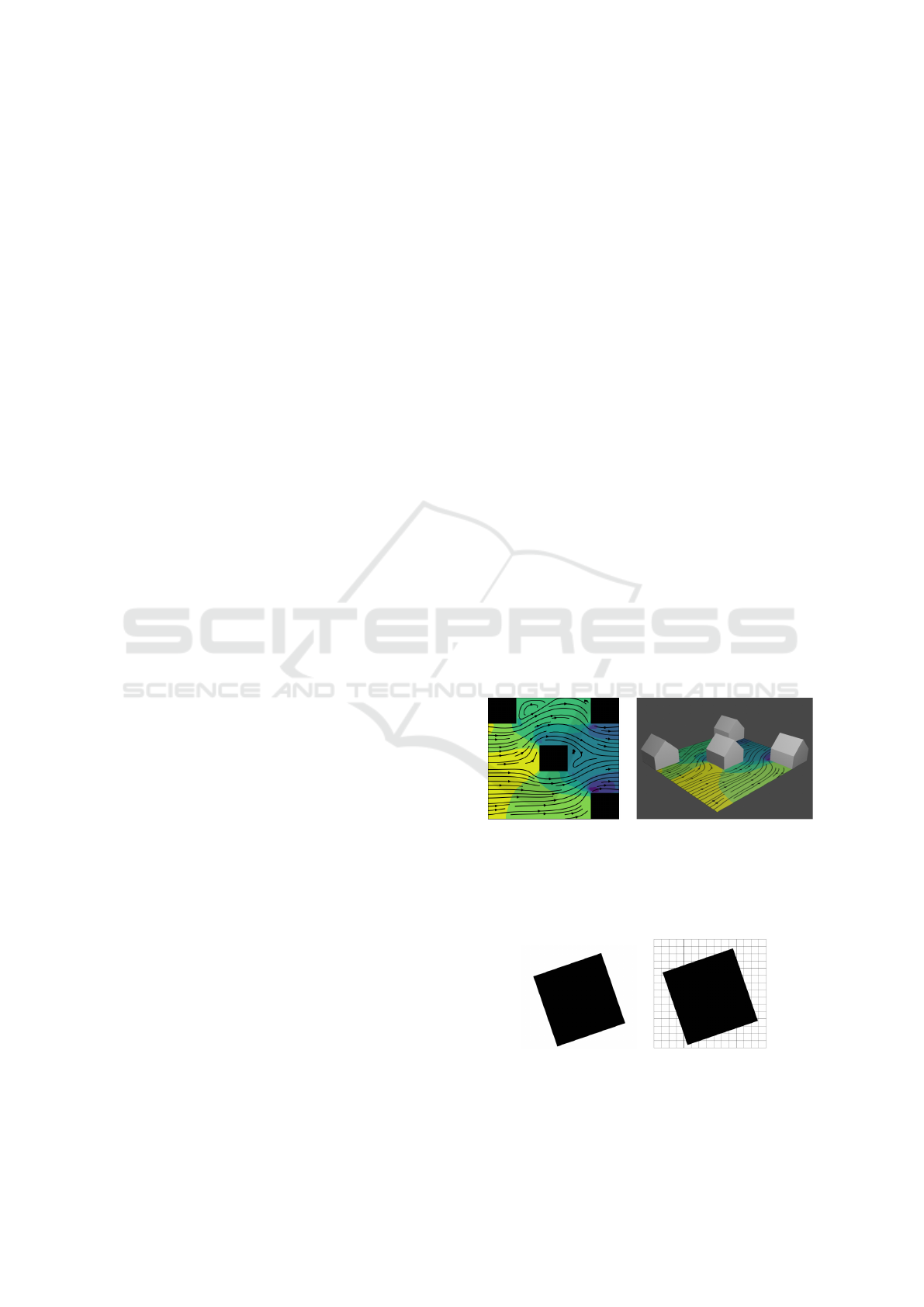
(a) (b)

Figure 2: Wind ﬂow and pressure: (a) A 2D scene with a

few buildings. (b) The same scene augmented by a more 3D

representation, a so-called quasi 3D visualization that adds

3D polygonal shapes on the buildings of the 2D representa-

tion to make it more understandable for the users.

(a) (b)

Figure 3: The 2D outline of a building (a) gets placed into

a grid consisting of equally sized grid cells (b).

Interactive Wind Simulation in Settlement Areas

825

4.2 Integrating Outlines into a Grid

In a ﬁrst step, we describe how an outline gets mapped

to a grid which requires an exact matching from the

building geometry to a corresponding grid of a cer-

tain resolution. Figure 3 illustrates a 2D model of a

building depicted as black square (a) that is placed

into a uniform grid of equally sized grid cells (b). It

may be noted that the resolution of the grid cannot

be inﬁnitely high due to the fact that each grid cell

will be treated as a separate variable in the physical

computation, i.e. more of them would cause more

complex computations resulting in a higher runtime

performance. For this reason, we need an adequate

resolution to allow live computations and hence, inter-

active responsiveness during the simulation process.

Each grid cell can only have one out of two states:

Either it belongs to a building or not, requiring a pre-

step before the simulation computation that checks

each grid cell for this property. To get a quick so-

lution to this problem we apply the Bresenham algo-

rithm (Angel and Morrison, 1991) that is able to draw

lines between the corners of the polygon modeling the

building outlines. Negatively, we soon get effects that

are well-known as pixel staircases in low resolution

images (see Figure 4).

Finally, we obtain a geometry that is compatible

with the simulation algorithm, i.e. we generate a so-

called ﬂag ﬁeld that we take into account in the com-

putation to judge whether a grid cell corresponds to a

piece of a building or not (see Figure 5).

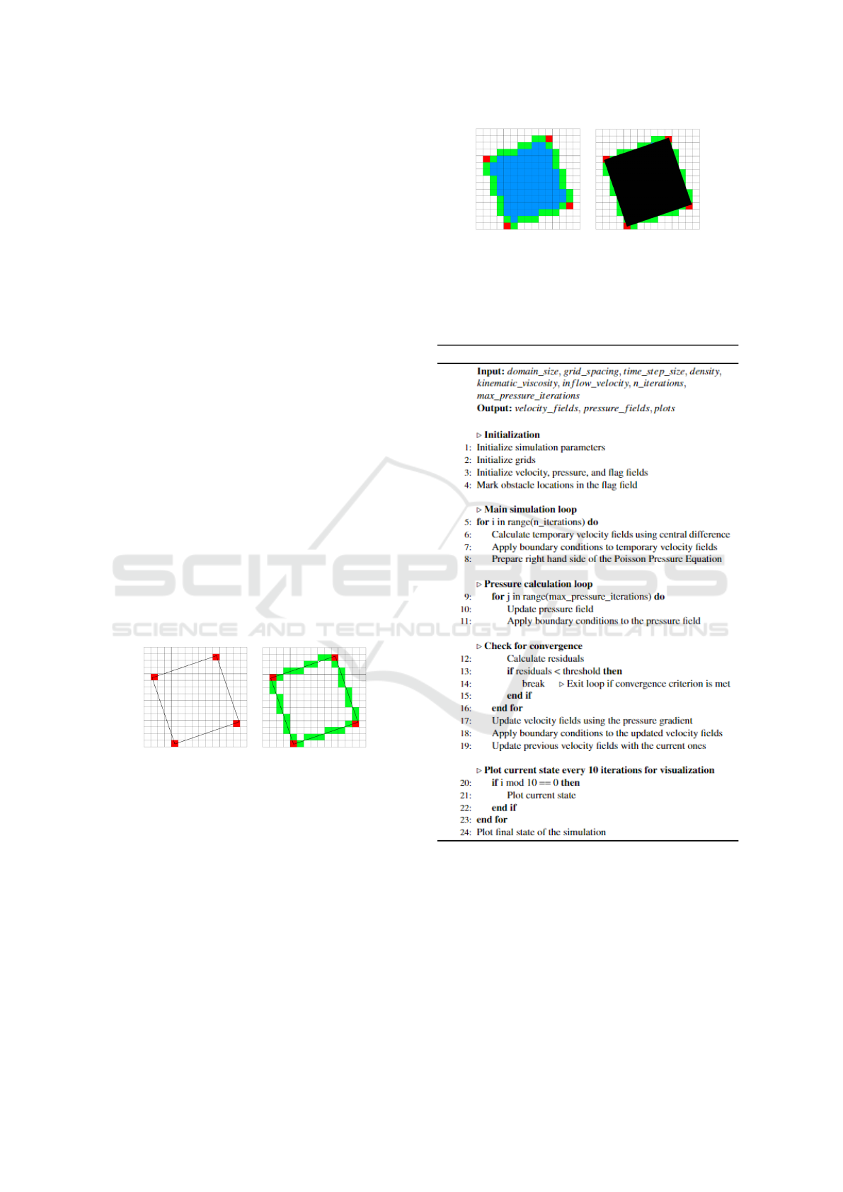
(a) (b)

Figure 4: Computing the corners (red squares) of the 2D

outline (a) and identifying the grid cells that are hit by the

corner-connecting lines (green squares) (b). This may result

in some kind of staircase effect.

4.3 Invalid Geometry

The computation of the simulation is problematic at

the walls and corners around an obstacle. We must

apply boundary conditions to follow physical laws

correctly. Otherwise, the wind might ﬂow through

walls or the pressure is incorrectly computed. Most

of the computation methods have such problems with

obstacle grid cells that have more than 2 free, direct

neighbors or that have free neighbors above and be-

low (which is a wall consisting of just one grid cell).

(a) (b)

Figure 5: An identiﬁed outline of a building depicted as

corners (red squares), outline connecting the corners (green

squares), and the inside (blue squares) (a). Overplotting

with the original 2D building shows the ﬁnal result in the

grid with the original shape (b).

Algorithm 1: The windy ﬂow simulation algorithm.

For this reason, we have to re-inspect all situ-

ations after the geometries have been computed to

avoid such negative and error-prone cases. Actually,

we have three options to avoid such cases:

• Grid Reﬁnement. We reﬁne the grid. If we split

the involved grid cell into 2 × 2 grid cells we

get rid of the problematic cell due to the fact that

it does not have 3 free neighbor cells anymore.

However, a new problem might be the increased

number of cells that can cause a more complex

IVAPP 2025 - 16th International Conference on Information Visualization Theory and Applications

826

(a) (b)

Figure 6: Reﬁning the grid due to the fact that there are

free neighbors causing problems in the physical correctness:

(a) One grid cell has 3 free neighbors. (b) Grid reﬁnement

avoids this situation.

(a) (b)

Figure 7: Two more options to get rid of the problematic

situation: (a) Local adaptation of the grid. (b) Removal of

the problematic grid cell.

and longer running computation (see Figure 6).

• Adaptive Grid. We adapt the grid by reﬁning it

only at locations in which invalid geometries ex-

ist. The beneﬁt of this approach is that we do not

need much more storage as in the general grid re-

ﬁnement, however as a drawback the storing pro-

cess would get much more complex due to the fact

that our data structures have to handle such special

situations (see Figure 7 (a)).

• Grid Cell Removal. Just removing the problem-

atic grid cell might be the simplest solution, how-

ever, the simulation will get less exact due to the

missing geo-spatial information. In most cases

such scenarios just occur for tiny pieces of houses

or obstacles, hence this solution might be the best

one, also because we have tested it in experiments

(see Figure 7 (b)).

It may be noted that the grid is discretized, ac-

tually allowing to make it inﬁnitesimally small but

due to the fact that we have to solve equation sys-

tems whose complexity depends on the number of in-

volved grid cells, we should avoid such a situation.

This means the buildings have to be downscaled to

make the simulation efﬁciently computable.

4.4 Algorithmic Performance

We tested our approach by applying it to a scenario

containing 150 × 150 grid cells, in total 22,500 cells.

The used hardware is a laptop with a CPU, a Mi-

crosoft Surface Laptop Studio processor Intel Core

i7-11370H, 4 core, 3 GHz and 16 GB RAM.

The visualizations will be shown as animation

which means they can be regarded as some kind of gif,

overplotting each image in the sequence by the next

one. The initialization lasts 2.4 to 3.5 seconds, but

this is independent from the ﬁnal performance. The

concrete measurements for the running program and

for 1,270 iterations and 127 visualizations are 2.7031

seconds for the initialization, 0.8409 seconds for the

mean time between visualizations, 0.0022 seconds

variance, 0.0468 seconds standard deviation, 1.0005

seconds maximum, and 0.7501 seconds minimum.

5 VISUALIZATION TOOL

To explore the results of the simulation algorithm we

created a visualization tool that can depict the results

in different visual encodings and views. Moreover, in-

teractions are supported to let users adapt parameters

or navigate in the visual results. Before implementing

the tool we started with a design phase including visu-

alization techniques and interactions as well as algo-

rithmic concepts. All of them are integrated and laid

out in a user interface.

We focus on the most prominent visualization

techniques for this kind of data. The visualizations

can be shown separately or as overlay on users’ de-

mands.

• Wind Flow. The wind ﬂow will be displayed

by streamlines, also showing the wind directions,

densities, and speed by arrow heads, proximity,

and frequency of arrow heads.

• Pressure. The pressure is visually depicted by a

contour plot using color coding to show the pres-

sure values in certain regions. We use a categori-

cal color scale here instead of a continuous one.

• Geography and Buildings. A geographic map

containing abstractions for the buildings provides

an overview about the geo-spatial data.

• 3D Augmentation: Quasi 3D depictions are use-

ful to better illustrate the geographical scene with

wind ﬂows and pressures and look more natural

and more aesthetically pleasing.

We integrate user interactions for modifying simu-

lation parameters and for directly impacting the visual

output (Yi et al., 2007).

Interactive Wind Simulation in Settlement Areas

827

(a) (b) (c) (d)

Figure 8: Visualizing the outcomes of the simulation for two scenarios: (a) shows streamlines for the wind direction overlaid

on a contour map depicting the pressure with a color coding. (b) We modiﬁed one building (top left) to compare the impact

on wind ﬂows and pressure. (c) Same scenario as in (a) but this time the wind comes from East and not from West as in (a).

In (d) we see again the modiﬁcation of one building and its impact on the wind ﬂow result.

(a) (b) (c) (d)

Figure 9: Visualizing the velocities of the wind ﬂows for different wind directions as well as different building outlines:

(a) Wind from West and standard buildings. (b) Wind from West and building extension. (c) Wind from East and standard

buildings. (d) Wind from East and building extension.

6 APPLICATION EXAMPLE AND

RESULTS

As some kind of stress test we applied our approach

to GIS data from Zurich in Switzerland with 50,750

buildings.

6.1 Simple Scenarios

Figure 8 shows before-after scenes for the results of

the simulation algorithm. The visualizations are com-

posed of streamlines (for wind directions and inten-

sities) and contour maps (for pressure values). Fig-

ures 8 (a) and (c) show the simulation result for dif-

ferent wind directions while the computation in Fig-

ures 8 (b) and (d) also show different wind directions

but this time the scenario was modiﬁed by extend-

ing one building (top left) with an additional build-

ing. Figures 8 (a) and (b) show the wind coming from

West while Figures 8 (c) and (d) show the simulation

computation for wind coming from East.

For the variants without building extension in Fig-

ures 8 (a) and (c), we can see that the wind is mov-

ing more smoothly in the upper left corner without

turbulent or eddy currents compared to Figures 8 (b)

and (d), apart from the fact that in Figure 8 (a) the

wind is moving in a diagonal (West-North) direction

but in Figure 8 (c) this is not the case. For the sce-

nario in Figure 8 (b) with the modiﬁed building we

see that the wind from West is moving around the new

building part while in Figure 8 (d) the wind from East

creates turbulent and eddy currents and swirls in the

upper left corner. For the pressure (the color coded

contours) we can also see some differences between

the scenarios. Comparing Figures 8 (a) and (b) for

the wind from West we ﬁnd stronger pressure regions

in the corner of the modiﬁed building. For the situ-

ations in Figures 8 (c) and (d) with the wind coming

from East we see that the pressure in the corner of the

extended building got much lower which might be a

hint for a quiet place in the garden to relax in cases the

wind comes from the East direction. It may be noted

that we are able to interactively modify those situa-

tions to explore the best shapes for new built houses,

for example to create wind-free zones. Such a sim-

ulation might be of particular interest for architects

who plan a new house based on the house owners’

demands.

Figure 9 depicts the same building situation as in

Figure 8 but in this case we focus on the wind speed

instead of the wind pressure. The color of the con-

tour plot indicates the strength of the wind in terms

of wind speed. We can see that the wind speed is ac-

tually the highest around the corners of the building

close to the direction from where the wind is coming.

Also in a wind channel between two buildings we can

see a higher wind speed than in the open environment

which is due to physical laws related to wind speed

and wind pressure.

Figure 10 shows another example with three

buildings while one building is a bit smaller than the

IVAPP 2025 - 16th International Conference on Information Visualization Theory and Applications

828

Figure 10: Three buildings while one is smaller than the

two others. The wind is coming from West. We can clearly

see the effect of the buildings on the wind.

(a) (b)

Figure 11: Buildings from Zurich and the impact of wind

ﬂows and the fact that buildings are removed: (a) A part

from Zurich while the wind is coming from East. (b) One

building is removed and the wind is coming from the West.

other two ones. The wind is coming from West and

we can directly spot the largest pressure right before

the buildings closer to the West. In general, the pres-

sure is always largest at the side of the building facing

the wind directly and lowest behind the building.

6.2 More Complex Scenarios

Figure 11 shows examples including more buildings

than the scenes before. Also some real-world build-

ings from areas in Zurich are taken into consideration

for this kind of wind simulation. Also different wind

settings were applied resulting in different ﬂows while

buildings are removed to get an impression about the

impact of new building environments.

In Figures 11 (a) and (b) we can easily detect that

the wind direction has an impact on the wind ﬂows

around the buildings as well as the pressure. In (c) we

detect that there are just some strong pressure regions

while the center area of this environment seems to be

a quiet place with not much wind and low pressure

(blue color). In (d) it seems as if the wind is strongest

when it is leaving the building environment (yellow

and red colors to the right hand side).

6.3 Open Challenges and Perspectives

We are aware of the fact that there are also limitations

of our approach, however we developed a solution to

this problem at hand and will further develop more

scalable and user-friendly versions of the tool. For

example, more interaction techniques should be inte-

grated in the future, also letting users modify more pa-

rameters to change algorithmic computations on-the-

ﬂy. There are also still some limitations with respect

to scalability issues regarding visual, perceptual, and

algorithmic issues. We are still experimenting with

the tool and the algorithms that we use as well as the

hardware could be enhanced in the future to get even

faster and even more interactive results.

7 CONCLUSION AND FUTURE

WORK

In this work, we investigated the research problem

of computing wind ﬂows in settlement areas with the

goal to create a model to understand such wind situ-

ations, for example before a new building is planned,

built, or just extended. We show the results of the sim-

ulations visually and let the users interactively change

wind directions or add, remove, replace buildings as

well as other obstacles while the simulation adapts

immediately to the new situation. To illustrate the

usefulness of our approach we applied it to GIS data

from Switzerland and showed some visual results of

the simulations under different conditions. For fu-

ture work we plan to extend our work by using bet-

ter hardware and more efﬁcient algorithms and paral-

lelization, in particular with a focus on interactive re-

sponsiveness. This means we might install the tool on

some kind of large high-resolution display to let sev-

eral experts explore the data in a collaborative manner

(LHRD). We also plan to conduct an expert user study

with city planners and architects, maybe also tracking

eye movements (Burch, 2022) of the users with the

goal to analyze their visual attention behavior.

Interactive Wind Simulation in Settlement Areas

829

REFERENCES

Angel, E. and Morrison, D. (1991). Speeding up bresen-

ham’s algorithm. IEEE Computer Graphics and Ap-

plications, 11(6):16–17.

Bader, M., Mehl, M., R

ude, U., and Wellein, G. (2011).

Simulation software for supercomputers. Journal of

Computational Science, 2(2):93–94.

Bryson, S. and Levit, C. (1992). The virtual wind tun-

nel. IEEE Computer Graphics and Applications,

12(4):25–34.

Burch, M. (2022). Eye Tracking and Visual Analytics. River

Publishers.

Burch, M., Wallner, G., Arends, S. T. T., and Beri, P.

(2020). Procedural city modeling for AR applications.

In et al., E. B., editor, Proceedings of the 24th Inter-

national Conference on Information Visualisation, IV,

pages 581–586. IEEE.

Chorin, A. J. (1967). Numerical solution of the navier-

stokes equations. Mathematics of Computation,

22:745–762.

Deininger, M. E., von der Gr

un, M., Piepereit, R., Schnei-

der, S., Santhanavanich, T., Coors, V., and Voß, U.

(2020). A continuous, semi-automated workﬂow:

From 3d city models with geometric optimization and

CFD simulations to visualization of wind in an urban

environment. ISPRS International Journal of Geo-

Information, 9(11):657.

Eidgenossenschaft, S. (2024). Bundesamt f

ur Landesto-

pograﬁe swisstopo.

Forney, G. P., Madrzykowski, D., McGrattan, K. B., and

Sheppard, L. (2003). Understanding ﬁre and smoke

ﬂow through modeling and visualization. IEEE Com-

puter Graphics and Applications, 23(4):6–13.

Kirkil, G. and Lin, C. (2020). Large eddy simulation of

wind ﬂow over A realistic urban area. Computation,

8(2):47.

Li, Y. and Zhao, H. (2023). Spatial wind ﬂow load and

shape optimization for folding grid shell buildings.

IEEE Access, 11:135304–135322.

Mayo, M., Wakes, S., and Anderson, C. (2018). Neural net-

works for predicting the output of wind ﬂow simula-

tions over complex topographies. In Wu, X., Ong, Y.,

Aggarwal, C. C., and Chen, H., editors, Proceedings

of the IEEE International Conference on Big Knowl-

edge, ICBK, pages 184–191. IEEE Computer Society.

Meinel, G. (2008). High resolution analysis of settlement

structure on base of topographic raster maps - method

and implementation. In Gervasi, O., Murgante, B., La-

gan

a, A., Taniar, D., Mun, Y., and Gavrilova, M. L.,

editors, Computational Science and Its Applications

- ICCSA 2008, International Conference, Perugia,

Italy, June 30 - July 3, 2008, Proceedings, Part I,

volume 5072 of Lecture Notes in Computer Science,

pages 16–25. Springer.

Papalexiou, S. and Moussiopoulos, N. (2006). Wind

ﬂow and photochemical air pollution in thessaloniki,

greece. part II: statistical evaluation of european

zooming model’s simulation results. Environmental

Modelling and Software, 21(12):1752–1758.

Paterson, D. and Apelt, C. (1989). Simulation of wind ﬂow

around three-dimensional buildings. Building and En-

vironment, 24(1):39–50.

Ridzuan, N., Ujang, U., and Azri, S. (2023). 3d vector-

ization and rasterization of citygml standard in wind

simulation. Earth Science Informatics, 16(3):2635–

2647.

Schlemmer, M., Hotz, I., Hamann, B., Morr, F., and Hagen,

H. (2007). Priority streamlines: A context-based visu-

alization of ﬂow ﬁelds. In Museth, K., M

oller, T., and

Ynnerman, A., editors, Proceedings of the 9th Joint

Eurographics - IEEE VGTC Symposium on Visualiza-

tion, EuroVis, pages 227–234. Eurographics Associa-

tion.

Seebacher, D., Miller, M., Polk, T., Fuchs, J., and Keim,

D. A. (2019). Visual analytics of volunteered geo-

graphic information: Detection and investigation of

urban heat islands. IEEE Computer Graphics and Ap-

plications, 39(5):83–95.

van Wijk, J. J. (1993). Flow visualization with surface par-

ticles. IEEE Computer Graphics and Applications,

13(4):18–24.

Wang, T., Wang, B., Matekole, E. S., and Atif, M. (2022).

Finding hidden patterns in high resolution wind ﬂow

model simulations. In Kothe, D. B., Geist, A.,

Pophale, S., Liu, H., and Parete-Koon, S., editors,

Proceedings of the Accelerating Science and Engi-

neering Discoveries Through Integrated Research In-

frastructure for Experiment, Big Data, Modeling and

Simulation - 22nd Smoky Mountains Computational

Sciences and Engineering Conference, SMC, Revised

Selected Papers, volume 1690 of Communications in

Computer and Information Science, pages 345–365.

Springer.

Wu, A., Deng, D., Chen, M., Liu, S., Keim, D. A., Ma-

ciejewski, R., Miksch, S., Strobelt, H., Vi

egas, F. B.,

and Wattenberg, M. (2023). Grand challenges in vi-

sual analytics applications. IEEE Computer Graphics

and Applications, 43(5):83–90.

Yan, Z., Chen, R., and Cai, X. (2022). Large eddy simu-

lation of the wind ﬂow in a realistic full-scale urban

community with a scalable parallel algorithm. Com-

puter Physics Communications, 270:108170.

Yang, Z., Sarkar, P., and Hu, H. (2010). Visualiza-

tion of ﬂow structures around a gable-roofed building

model in tornado-like winds. Journal of Visualization,

13(4):285–288.

Yi, J. S., ah Kang, Y., Stasko, J. T., and Jacko, J. A.

(2007). Toward a deeper understanding of the role

of interaction in information visualization. IEEE

Transactions on Visualization and Computer Graph-

ics, 13(6):1224–1231.

Yin, J., Zhan, Q., Xiao, Y., Wang, T., Che, E., Meng, F.,

and Qian, Y. (2014). Correlation between urban mor-

phology and wind environment in digital city using

GIS and CFD simulations. International Journal of

Online Engineering, 10(3):42–48.

Zu, G. and Lam, K. M. (2018). LES and wind tunnel test

of ﬂow around two tall buildings in staggered arrange-

ment. Computation, 6(2):28.

IVAPP 2025 - 16th International Conference on Information Visualization Theory and Applications

830