Indoor Navigation: Navmesh Applied to Indoor Graph Creation

Maxime Callico

1, 2

, Rodolphe Giroudeau

, Benoît Darties

and Jean Carrière

LIRMM, Montpellier, France

Woosmap, Montpellier, France

Keywords:

Navmesh, Graph, Shortest Path, Polygon, Convex, Concave, Indoor, Navigation.

Abstract:

This paper explores the adaptation of the Navmesh algorithm, widely used in video games for pathﬁnding,

to real-world indoor navigation. By applying polygon decomposition techniques, we generate routing graphs

for complex indoor environments. Our results demonstrate that the algorithm is particularly efﬁcient with

orthogonal polygons, commonly found in real-life buildings, due to their structured geometry. We compare

the performance across various polygon types and discuss optimization strategies for path naturalness and

computational efﬁciency. This work opens pathways for practical applications in indoor navigation.

1 INTRODUCTION

Indoor navigation has become increasingly signiﬁcant

as spaces like shopping malls, airports, and museums

grow more complex alongside societal advancements

(Diakité and Zlatanova, 2018). Companies currently

provide map services through terminals to help users

locate destinations, but the next step involves real-

time positioning and navigation within these environ-

ments.

This research focuses on generating graphs for in-

door route searches. Presently, maps are manually an-

notated with location data (e.g., train stations, stores),

and vertices are placed at ﬁxed intervals, leading to

dense graphs. Automating this process with polygon

division algorithms could reduce workloads while of-

fering tailored routing solutions based on different ob-

jective functions.

The main goal is to develop an optimal strategy

for creating indoor navigation graphs using Open-

StreetMap (OSM) data. This study adapts the

Mesh Navigation (Navmesh) algorithm proposed by

(Oliva and Pelechano, 2011), which partitions non-

intersecting polygons into convex subsets. Although

Navmesh is widely used in video games (Snook,

2000), this project applies it to indoor navigation.

Unlike road maps, where vertices naturally rep-

resent intersections and edges correspond to roads,

indoor spaces present challenges. Placing vertices

at regular intervals produces overly dense graphs,

while positioning them at entrances/exits fails for

non-convex rooms. A single vertex per room simpli-

ﬁes the graph but yields unrealistic routes. Navmesh,

however, efﬁciently partitions complex spaces into

routing graphs for realistic navigation, a technique

adapted here.

The algorithm presented in (Oliva and Pelechano,

2011) has limitations: it omits the processing order

for concave angles and assumes minimizing polygons

as its goal without clear justiﬁcation. This work ex-

plores multiple objective functions to assess the best

approach.

The project begins with implementing the algo-

rithm and conducting tests to evaluate its parameters,

identify limitations, and optimize performance.

The remainder of this paper is organized as fol-

lows: Section 2 reviews related work, Section 3 de-

tails the Navmesh algorithm, Section 4 compares it to

other methods, Section 5 presents results, and Section

6 offers concluding remarks.

2 RELATED WORK

While a signiﬁcant amount of literature focuses on the

modelization of indoor navigation graphs (Park et al.,

2020)(Zhou et al., 2022)(Noureddine et al., 2020),

fewer works address their automatic generation. The

emphasis often lies on describing models rather than

automating their creation. This gap highlights the

need for more research into methods for automatic

graph generation.

The division of polygons into convex components

is not a new concept. It has been applied to nav-

Callico, M., Giroudeau, R., Darties, B. and Carrière, J.

Indoor Navigation: Navmesh Applied to Indoor Graph Creation.

DOI: 10.5220/0013109800003893

Paper published under CC license (CC BY-NC-ND 4.0)

In Proceedings of the 14th International Conference on Operations Research and Enterprise Systems (ICORES 2025), pages 221-228

ISBN: 978-989-758-732-0; ISSN: 2184-4372

221

igation since the 1980s in robotics under the term

meadow mapping, introduced by Ronald C. Arkin

(Arkin, 1986). Theoretically, Lingas et al. (1982)

showed that dividing a polygon without holes can

be solved in O(n

) time, where n is the polygon’s

number of sides. Numerous other algorithms for

polygon decomposition have been formalized (Her-

tel and Mehlhorn, 2006) (Keil, 2000) (O’Rourke and

Supowit, 1983).

Since the early 2000s, the term Navmesh, of-

ten attributed to Golodetz (Snook, 2000), has gained

prominence, particularly as a pathﬁnding tool in video

games. Navmesh divides the walkable plane into con-

vex polygons to form a simple graph, producing natu-

ral paths. Extensive research exists on Navmesh gen-

eration for multi-story terrains, dynamic 3D environ-

ments (O’Rourke and Supowit, 1983) (Berseth et al.,

2015), real-time applications (Hale et al., 2021) and

pathﬁnding (Brewer, 2019). However, applying such

complex algorithms to 2D ﬂoor plans—simpler than

video game environments—would be inefﬁcient for

this work.

While methods for manually creating efﬁcient

routing graphs exist (Yuan and Schneider, 2010)

(Jensen et al., 2009), this study seeks an auto-

mated, straightforward approach. The algorithm from

(Oliva and Pelechano, 2011), which offers polyno-

mial complexity, has been chosen. Although generat-

ing Navmesh is NP-hard when minimizing polygons

(Keil, 2000), the resulting solution, while not optimal,

will be shown to be sufﬁcient for our needs.

3 NAVMESH

In this section, the algorithm presented in (Oliva and

Pelechano, 2011) is described, followed by an exam-

ple that illustrates the creation of the graph through

polygon division.

3.1 Description of the Algorithm

Let A = (a

,...,a

n−1

) be the considered polygon.

Let B = (b

,..., b

m−1

) be the set of non-convex

vertices of the polygon.

Deﬁnition 1 (Trigonometric and Anti-Trigonometric

Direction). A set of points in R

is in the trigonomet-

ric (resp. anti-trigonometric) direction if the points

are in an anti-clockwise (resp. clockwise) manner.

Deﬁnition 2 (Reﬂex Angles). Let α be an angle. α is

a reﬂex angle if α > π.

The goal of the algorithm is to divide the polygon

into a partition of convex polygons. The ﬁrst stage

Figure 1: Examples of angles. α is a reﬂex angle (

3π

> π)

but β is not (

involves identifying the reﬂex angles within the poly-

gon. To achieve this, we iterate over the vertices in

the anti-trigonometric direction. For each vertex a

we consider the triangle formed by a

i−1

, a

, and a

i+1

If the triangle lies in the external polygon (resp. in-

ternal polygon) and is in the anti-trigonometric (resp.

trigonometric) direction, then vertex a

has a reﬂex

angle.

To detect these angles, we use the signed area

of a triangle, calculated with the shoelace formula

(Braden, 1986). The signed area determines whether

the triangle is oriented in the anti-trigonometric di-

rection (strictly negative), the trigonometric direction

(strictly positive), or if the points are collinear (equal

to 0). Using this formula, we identify all reﬂex angles

in the polygon.

Once the concave vertices are identiﬁed, the algo-

rithm generates a set of portals. These portals divide

the vertex into two interior angles that are no longer

reﬂex. We ﬁrst describe the portal creation process

and then analyze the impact of the order in which con-

cave vertices are processed.

Deﬁnition 3 (Concave Vertex). A concave vertex is a

vertex of the original polygon in which interior angle

is a reﬂex angle. It is also called a notch.

An example of a concave vertex is presented in

Figure 1. α, which is a reﬂex angle, would be a con-

cave vertex if it was an internal angle inside a poly-

gon.

Let b

be in B. In this part, we will suppose all

indices are written modulo n −1. First of all, we have

to ﬁnd the interest area of b

Deﬁnition 4 (Interest Area). The interest area of a

vertex b

is the interior polygon formed by the exten-

sion of its two adjacent sides, e

i−1,i

and e

i,i+1

An example of interest area can be found in Figure

2. In that interest area, any straight line coming from

the vertex b

will divide the reﬂex angle into two non-

reﬂex angles. The object chosen by the algorithm,

i.e. the object closest to the concave vertex inside

of the interest area, will be connected to b

, correcting

his reﬂex angle.

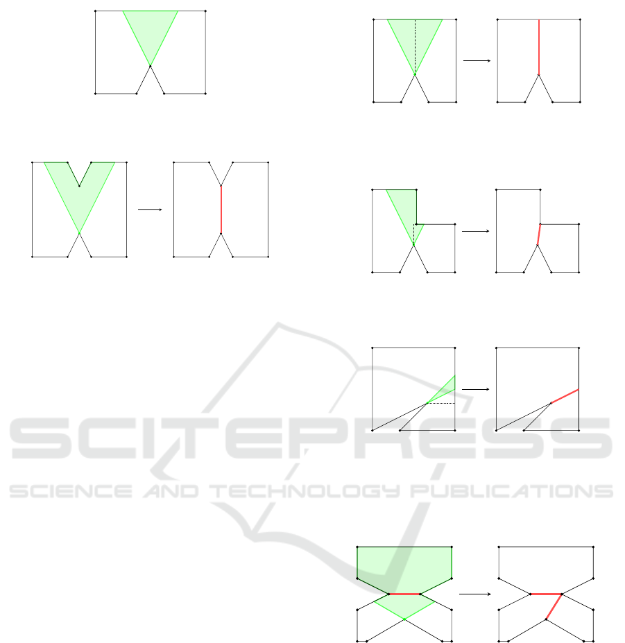
Depending on the closest object, there are three

possible cases:

ICORES 2025 - 14th International Conference on Operations Research and Enterprise Systems

222

i−1,i

i−1

i+1

Figure 2: Interest area example. The interest area I

, colored

in green, is the interest area of v

i−1,i

j−1, j

j, j+1

i−1

i+1

Figure 3: Portal from a vertex to another vertex. The closest

element to b

in the interest area I

is v

. On the right, the

resulting portal connecting the two, in red.

• if the closest object is another vertex c

, the por-

tal is simply a line between these two vertices. An

example of these kind of portals is found in 3.

• If the closest object is a side of the polygon e

there are ﬁve candidates for the portal. The clos-

est choice is its projection, but it is not necessarily

in the interest area. We can also consider the two

vertices incident to e

or the two intersections of

the interest area with e

. Figure 4 shows all possi-

ble cases of this step.

• Lastly, if the object is another portal P

, we con-

nect the vertex to the closest extremity of P

. If

none of these extremities are in the interest area,

we connect it to both of the extremities of the por-

tal. Two examples are shown in 5.

We now know what to do with each concave ver-

tex of the polygon. The question becomes: In which

order are we going to consider the vertices?There are

multiple possible orders:

• Random Order: the random order is the ﬁrst

possibility. We think adding a random dimension

could allow to better the performances instead of

blindly following the same order for each poly-

gon.

• Trigonometric Order: it would be interesting to

compare the performances to a default order like

this one.

• Biggest (or Smallest) Angle First: dividing the

biggest angles ﬁrst could give us bigger polygons

from which to create the graph, but smallest inter-

est areas gives us less choice, accelerating perfor-

mance at the cost of some other characteristics.

i−1,i

i,i+1

i−1

i+1

(a) Portal from a vertex to a side of the polygon. On the

left, the considered polygon, with b

the current vertex and

the interest area. The projection of e

is the closest object

in the area, so the portal on the right connects the two.

i−1,i

i,i+1

(b) Portal from a vertex to a side of the polygon. The pro-

jection is not in the interest area; the closest object to b

the extremity of e

, so on the right the two objects are con-

nected.

i−1,i

i,i+1

jection is not in the interest area; the closet object in the

interest area is the intersection between the extension of

i−1,1

. On the right, the two objects connected.

Figure 4: Portals from a vertex to a side of the polygon.

i−1,i

i,i+1

Figure 5: Portal from a vertex to another portal. On the

left, we see the portal p

is the closest object to b

inside its

interest area; both extremities are at the same distance, so

we can chose one at random and connect it to b

, which is

done on the right.

3.2 Description of the Graph

From the division of the polygon in its different con-

vex parts, we can create the graph by adding a node

for every portal and creating a visibility graph.

Deﬁnition 5 (Visibility Graph in a Polygon). Let P be

a polygon. Let V be a set of nodes inside of the poly-

gon. We create E = {(i ∈ V, j ∈ V ),P covers (i, j)}.

Indoor Navigation: Navmesh Applied to Indoor Graph Creation

223

The visibility graph for the nodes V in P is G = (V,E).

The visibility graph contains an edge between ev-

ery two vertices that can see each other; in other

words, it contains an edge between every two vertices

whose edge would be contained inside the polygon.

For our graph, we also add the condition that a

portal acts as an edge of the polygon, i.e. an edge

of the graph would not cross the portals. The next

section contains examples of graph creation.

4 COMPARISON

In this section, we compare the Navmesh method to

other commonly used approaches for indoor graph

generation. Navmesh, while originally developed for

video game pathﬁnding, has demonstrated signiﬁcant

potential for real-world applications, such as indoor

navigation in complex environments. However, sev-

eral alternative methods exist, each with their own ad-

vantages and drawbacks.

4.1 Equidistant Nodes

An alternative approach for graph creation involves

covering the polygon with evenly spaced nodes and

connecting adjacent nodes with arcs. As shown in

Figure 6, the graph produced by Navmesh is notably

less dense in comparison. While the equidistant nodes

method is not inherently ﬂawed, it results in overly

dense graphs, which signiﬁcantly increase the com-

putational cost of ﬁnding the shortest path.

4.2 Delaunay Triangulation

Another way of creating the graph is using Delaunay

triangulation (Delaunay, 1934). If we triangulate the

polygon in that way, we can obtain different portals,

and we can create the graph using the same method

used for Navmesh.

Figure 7 shows us a comparison between these

two methods. Density is no longer a problem, but

one of our main goals is the "naturalness of the path",

i.e., that the path chosen in the graph should be as

close as possible to what a human would do. We

see in the Delaunay triangulation graph, the paths we

could ﬁnd would have a number of π/2 turns, but the

graph generated by Navmesh would, intuitively, ﬁnd

more natural paths.

(a) Graph created by Navmesh.

(b) Graph created using equidistant nodes.

Figure 6: Comparison between Navmesh and the equidis-

tant nodes method.

5 PRACTICAL RESULTS

5.1 Theoretical Results

This section presents the obtained results. The algo-

rithm has been applied to a set of three different types

of polygons, each varying in size:

• Normal polygons - the algorithm was applied to

randomly generated normal polygons to establish

a performance baseline.

• Orthogonal polygons - these polygons are com-

posed exclusively of 90-degree or 270-degree an-

gles. Intuitively, orthogonal polygons are unions

of rectangular shapes.

• Isothetic polygons - isothetic polygons are con-

structed using two distinct families of lines, where

each family passes through a different common

point, forming a skewed grid.

Figure 8 represents an example of both an orthog-

onal polygon and an isothetic polygon.

ICORES 2025 - 14th International Conference on Operations Research and Enterprise Systems

224

(a) Graph created by Navmesh.

(b) Graph created using Delaunay triangula-

tion.

Figure 7: Comparison between Navmesh and the Delaunay

triangulation method.

(a) (b)

Figure 8: On a, an orthogonal polygon, created from a

quadrilateral grid. On (b, an isothetic polygon, formed from

the grid created by two different families of lines passing

through the same common point.

5.1.1 Polygon Generation

To create the test sets, a random number of polygons

was generated using two different polygon genera-

tion methods. For the normal polygons, no restric-

tions were imposed, except for the exclusion of self-

intersecting polygons. The used method allows for

the generation of any polygon, including those with

holes. The technique employed, known as Inward

Denting, is derived from the article "Approaches for

Generating 2D Shapes." (Hada, 2014).

Normal Polygons. The ﬁrst step in generating nor-

mal random polygons involves selecting n random

points, where n represents the number of vertices in

the ﬁnal polygon. The randomness of the polygon

arises from these points, as the algorithm itself is de-

terministic and will produce the same polygon when

given the same set of points.

Initially, the convex hull of the set of points must

be determined. Several convex hull algorithms can

be employed for this task, such as the Gift Wrapping

algorithm (Jarvis march) (Jarvis, 1973), or Chan’s al-

gorithm (Chan, 1996). However, this article will not

focus on this aspect.

The subsequent step, which is repeated until no

points remain outside the polygon, involves adding

the node that modiﬁes the perimeter the least. For

each arc of the polygon, the distance to each point is

computed, and the point that contributes the smallest

increase to the perimeter is added, while ensuring the

polygon remains non-intersecting.

Orthogonal and Isothetic Polygons. For orthogo-

nal polygons, we use the cut and expand method pro-

posed in (Tomás and Bajuelos, 2004). The genera-

tion of orthogonal polygons begins with a 2 × 2 grid,

where the grid is considered as a 2 × 2 square. From

this starting point, the grid is expanded, and random

sections are removed to generate an orthogonal poly-

gon. The algorithm is divided into two distinct steps:

the expand step selects a row and column of the grid

for expansion, while the cut step selects one of the

newly created areas to be removed.

When we generate orthogonal polygons on a grid

like in our method, we simply create a grid which can

be transformed into a matrix of size n × n with ones

where the polygon has a square and zeroes where it

does not. For isothetic polygons, we can then generate

the isothetic grid and use that matrix as a template for

that grid.

5.1.2 Results

Tests were executed on a server with 8GB of RAM

and an Intel(R) Xeon(R) with 2.50GHz. The algo-

rithm has been coded in Python; the importance of the

results lies mostly on the comparison between perfor-

mances, more so than on the performance itself.

To begin with, tests on three different types of

polygons, described above with different sizes, rang-

Indoor Navigation: Navmesh Applied to Indoor Graph Creation

225

ing from 20 to 500 nodes per polygon, with 20 poly-

gons generated for each size, are executed. The means

are represented in the graph.

The results in Figure 9 show the performance of

the Navmesh algorithm across normal, orthogonal,

and isothetic polygons of varying sizes. Orthogonal

polygons consistently demonstrate the fastest com-

putation times, even as size increases. This is due

to their simple geometry, which minimizes the need

for complex subdivisions and enables efﬁcient space

partitioning. Since orthogonal polygons often repre-

sent real-world structures like grid-based buildings,

these results highlight the practical applicability of

Navmesh in such environments. Additionally, the

tight error bars indicate consistent performance across

trials, conﬁrming the robustness of the algorithm for

this polygon type.

In contrast, normal and isothetic polygons exhibit

signiﬁcantly longer computation times as size grows.

Normal polygons, with their irregular shapes, re-

quire more subdivisions to ensure convexity, increas-

ing processing time. Isothetic polygons, despite be-

ing theoretically regular, often introduce small, com-

plex geometries as they scale, contributing to sub-

stantial variability. This variability is evident in their

wider error bars, suggesting less predictable perfor-

mance. These ﬁndings emphasize the computational

challenges of irregular geometries and the importance

of selecting appropriate polygon types for efﬁcient

Navmesh execution in real-world applications.

The next tests, shown in Figure 10 are about the

order of the nodes. The original article does not talk

about the order: we take the interest areas of the

notches and we ﬁnd for each notch its closest element,

but we don’t know in which order the notes are con-

sidered. For this test, we compute how many portals

were added when considering the same polygon using

different orders. We have considered ﬁve different or-

ders:

• Normal Order: Notches are processed in a

clockwise order around the polygon.

• Random: Notches are processed in a randomly

determined order.

• Biggest or Smallest Angles First: Notches are

ordered by their internal angle size, with the

largest (or smallest) angles being processed ﬁrst.

The results show that normal and random pro-

cessing orders perform similarly, with no signiﬁcant

difference in the number of portals added. How-

ever, starting with the smallest angles increases portal

count, especially for larger polygons, as small inter-

nal angles create complex subdivisions early. In con-

trast, prioritizing larger angles simpliﬁes the problem

earlier, reducing subdivisions. Regardless of order,

portal count grows linearly with polygon size.

For random polygons, the results highlight

promising real-world applications. Orthogonal poly-

gons, common in real buildings, compute signiﬁ-

cantly faster. Additionally, processing the largest an-

gles ﬁrst reduces portal count and graph density, im-

proving shortest-path search efﬁciency. These ﬁnd-

ings are encouraging for practical use cases.

5.2 Real Use Cases

As part of the investigation, a program was developed

to apply the algorithm to real-world cases. By using

a GeoJSON ﬁle representing a real building as input,

the program executes the algorithm on the building

and generates a graph, which is then provided to the

user.

Deﬁnition 6 (GeoJSON File). A GeoJSON ﬁle is a

digital document containing geographical informa-

tion in the form of polygons, lines, or points. The data

is represented in terms of latitude and longitude.

The graphs generated for real-world scenarios are

both natural and accurately reﬂect the underlying en-

vironment. Figure 11 illustrates an example of a real-

world case processed by the program. The portals

generated are not excessive, and the resulting path

appears natural and intuitive. This outcome demon-

strates the effectiveness of the algorithm in produc-

ing paths that closely mirror real-world navigation

patterns, avoiding the creation of overly complex or

unnatural routes while ensuring computational efﬁ-

ciency.

6 CONCLUSION

This paper shows that the Navmesh concept, widely

used in video games, can be adapted to real-world en-

vironments. The proposed algorithm balances com-

putational complexity and practical use, even with the

NP-hard challenge of polygon division. While not al-

ways optimal, the results prove effective for real-life

cases, especially with simpler structures.

Tests reveal the algorithm performs best on or-

thogonal polygons, typical of real-world buildings,

thanks to their regularity, which simpliﬁes the search

space and reduces execution time. Irregular polygons,

on the other hand, increase complexity as their size

grows. Still, the algorithm remains scalable and efﬁ-

cient, even for larger inputs.

Node processing tests showed that prioritizing the

largest angles reduces portal count, with all orders

ICORES 2025 - 14th International Conference on Operations Research and Enterprise Systems

226

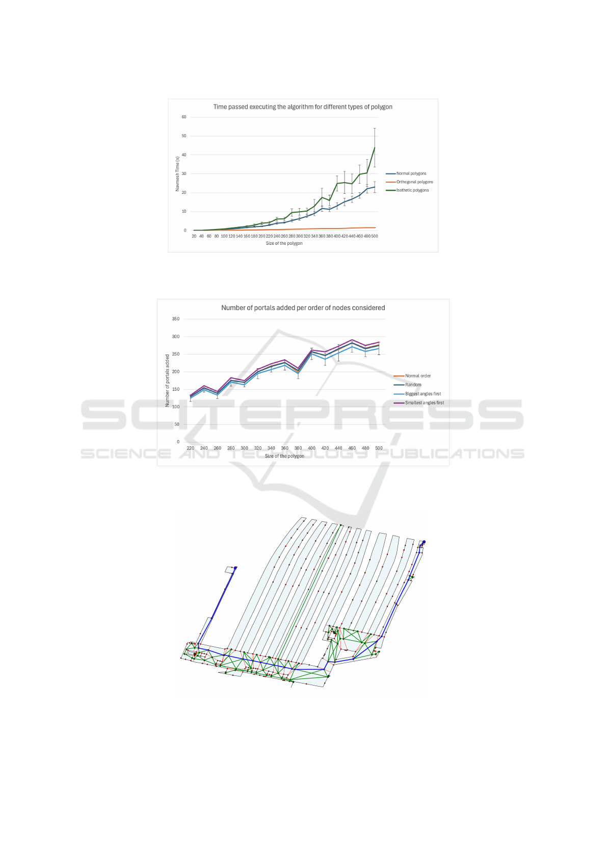
Figure 9: Time spent executing the Navmesh algorithm across different polygon types and sizes. The error bars represent the

95% conﬁdence interval for the results. Isothetic polygons exhibit signiﬁcantly greater variability while orthogonal polygons

maintain consistently lower and more stable computation times, with barely visible conﬁdence intervals.

Figure 10: Number of portals added per node order considered. The conﬁdence intervals for the biggest angles ﬁrst strategy

are shown: 95% of the values obtained in our simulations fall within 15% of the value represented on the plot. There are two

middle bars, representing the normal and random values, which have very similar values.

Figure 11: Application of the algorithm to a real use case. In red, the portals created by the algorithm, and in green the

generated graph. In blue, a found shortest path crossing the station.

Indoor Navigation: Navmesh Applied to Indoor Graph Creation

227

maintaining linear growth. Future work will focus on

improving path “naturalness” and optimizing for real-

ism over speed to ensure intuitive navigation solutions

across various polygon types.

Future research will focus on applying this

method to real-world scenarios and further investigat-

ing the “naturalness” of paths. Since the number of

portals directly impacts the graph, future work could

aim to optimize for path realism over speed, ensuring

intuitive and context-appropriate navigation solutions

across various polygon types.

REFERENCES

Berseth, G., Kapadia, M., and Faloutsos, P. (2015). Ac-

clmesh: Curvature-based navigation mesh generation.

In Proceedings of the 8th ACM SIGGRAPH Confer-

ence on Motion in Games, page 97–102.

Braden, B. (1986). The surveyor’s area formula. The Col-

lege Mathematics Journal, 17(4):326–337.

Brewer, D. (2019). Tactical pathﬁnding on a navmesh.

Game AI Pro, 360:25–32.

Chan, T. M. (1996). Optimal output-sensitive convex hull

algorithms in two and three dimensions. Discrete &

Computational Geometry, 16(4).

Delaunay, B. (1934). Sur la sphère vide. Bulletin de

l’Academie des Sciences de l’URSS. Classe des sci-

ences mathematiques et na, 1934(6):793–800.

Diakité, A. A. and Zlatanova, S. (2018). Spatial subdivi-

sion of complex indoor environments for 3d indoor

navigation. International Journal of Geographical In-

formation Science, 32(2):213–235.

Hada, P. S. (2014). Approaches for generating 2d shapes.

UNLV Theses, Dissertations, Professional Papers,

and Capstones.

Hale, D. H., Youngblood, G. M., and Dixit, P. (2021).

Automatically-generated convex region decomposi-

tion for real-time spatial agent navigation in virtual

worlds. In Proceedings of the AAAI Conference on Ar-

tiﬁcial Intelligence and Interactive Digital Entertain-

ment, pages 173–178.

Hertel, S. and Mehlhorn, K. (2006). Fast triangulation of

simple polygons. In Lecture Notes in Computer Sci-

ence, pages 207–218.

Jarvis, R. (1973). On the identiﬁcation of the convex hull

of a ﬁnite set of points in the plane. Information Pro-

cessing Letters, 2(1).

Jensen, C. S., Lu, H., and Yang, B. (2009). Graph model

based indoor tracking. In Proceedings - IEEE In-

ternational Conference on Mobile Data Management,

pages 122–131.

Keil, J. M. (2000). Polygon decomposition. Handbook of

computational geometry, 2:491–518.

Noureddine, H., Ray, C., and Claramunt, C. (2020). Seman-

tic trajectory modelling in indoor and outdoor spaces.

In 2020 21st IEEE International Conference on Mo-

bile Data Management (MDM), pages 131–136.

Oliva, R. and Pelechano, N. (2011). Automatic generation

of suboptimal navmeshes. In MIG’11: Proceedings of

the 4th International Conference on Motion in Games,

pages 328–339.

O’Rourke, J. and Supowit, K. (1983). Some np-hard poly-

gon decomposition problems. IEEE transactions on

information theory, 29:181–190.

Park, J., Goldberg, D. W., and Hammond, T. (2020). A com-

parison of network model creation algorithms based

on the quality of wayﬁnding results. Transactions in

GIS, 24(3):602–622.

Snook, G. (2000). Simpliﬁed 3d movement and pathﬁnd-

ing using navigation meshes. In Game Programming

Gems, pages 288–304. Charles River Media.

Tomás, A. P. and Bajuelos, A. L. (2004). Generating ran-

dom orthogonal polygons. In Current Topics in Artiﬁ-

cial Intelligence, pages 364–373, Berlin, Heidelberg.

Yuan, W. and Schneider, M. (2010). inav: An indoor

navigation model supporting length-dependent opti-

mal routing. In Lecture Notes in Geoinformation and

Cartography, pages 299–313.

Zhou, Z., Weibel, R., Richter, K.-F., and Huang, H. (2022).

Hivg: A hierarchical indoor visibility-based graph for

navigation guidance in multi-storey buildings. Com-

puters, Environment and Urban Systems, 93:101751.

ICORES 2025 - 14th International Conference on Operations Research and Enterprise Systems

228