Oasis: A Real-Time Hydraulic and Aeolian Erosion Simulation with

Dynamic Vegetation

Alexander Maximilian Nilles

, Lars G

unther and Stefan M

uller

Institute for Computational Visualistics, University of Koblenz, Universit

atsstr. 1, Koblenz, Germany

{nillesmax, larsguenther98, stefanm}@uni-koblenz.de

Keywords:

Real-Time Simulation, Aeolian Erosion, Hydraulic Erosion, Vegetation Simulation, Desert, Sand Dune

Simulation, GPU, CUDA.

Abstract:

We present a novel real-time combined simulation for aeolian erosion, hydraulic erosion and vegetation, ca-

pable of transforming barren deserts with sand dunes into lush forest landscapes and vice versa using simple

user interaction. Existing aeolian and hydraulic erosion methods are extended and uniﬁed using a moisture

model on a layered heightmap, supporting bedrock, soil and sand as terrain materials. Vegetation uses a 3D

radius-based model and is efﬁciently rasterized to a 2D density map via a split-Gaussian model, inhibiting

erosion. Abiotic factors such as moisture, terrain slope, surface water and illumination are considered in veg-

etation growth and vegetation can spread radially as well as with the wind. Each plant considers the position

and size of all neighboring plants as a biotic growth factor, made possible through a set of uniform grids of

varying resolutions. The user can freely model different plant species by deﬁning their ecological niche and

adaptability to changes in terrain elevation and competition with other plants. Even underwater vegetation is

possible. Interspecies competition can be deﬁned freely using a competition matrix. The resulting method

runs in real-time at a terrain resolution of 2048

with 2,000,000.00 plants.

1 INTRODUCTION

Erosion processes play a key role in landscape forma-

tion, which is an important area of computer graph-

ics. Real-time erosion simulations on heightmaps ex-

ist for both hydraulic (water-based) erosion (Benes,

2007; Mei et al., 2007; Kri

stof et al., 2009;

St’ava

et al., 2008) and aeolian (wind-based) erosion (Taylor

and Keyser, 2023; Nilles et al., 2024a), however, to

the best of our knowledge, no method currently ex-

ists that combines hydraulic and aeolian erosion with

support for dune propagation in a single simulation.

Vegetation, which interacts bidirectionally with

terrain, is also important to landscapes. Plenty of re-

search in computer graphics has dealt with placing

large amounts of vegetation in a plausible or realis-

tic manner on existing landscapes. Some real-time

erosion simulations also consider the effects of veg-

etation on erosion, but do not simulate the vegeta-

tion itself, such as in (Hawkins and Ricks, 2023).

However, non-real-time methods combining erosion

and vegetation bidirectionally have been proposed be-

fore (Cordonnier et al., 2017). This method in partic-

https://orcid.org/0000-0002-4196-7424

ular, while interactive and powerful, requires almost

an entire minute for a simulation step at a low res-

olution. In the current time, higher resolutions are

usually required and long waiting periods for a poten-

tially undesired result from the viewpoint of an artist

are likely to cause such methods to be rejected in this

ﬁeld.

In this paper, we propose a novel method that ﬁlls

both gaps. Our method combines aeolian and hy-

draulic erosion with a vegetation simulation. We sim-

ulate vegetation growth and spread while consider-

ing biotic and abiotic factors. All simulation compo-

nents affect each other bidirectionally, which is made

possible using a terrain moisture model and a split-

Gaussian rasterization of our novel radius-based veg-

etation model. Our method is fully interactive and the

user can change parameters to transform a desert into

a lush forest and vice versa, or create an oasis in a

desert. The method is capable of simulating a 2048

sized terrain with two million plants in real-time. It is

the ﬁrst method in computer graphics that simulates

aeolian erosion, hydraulic erosion and vegetation in a

bidirectional manner in real-time at this scale. To fa-

cilitate reproduction of our results, the code is avail-

able open source (Nilles and G

unther, 2025).

Nilles, A. M., Günther, L. and Müller, S.

Oasis: A Real-Time Hydraulic and Aeolian Erosion Simulation with Dynamic Vegetation.

DOI: 10.5220/0013112100003912

Paper published under CC license (CC BY-NC-ND 4.0)

In Proceedings of the 20th International Joint Conference on Computer Vision, Imaging and Computer Graphics Theory and Applications (VISIGRAPP 2025) - Volume 1: GRAPP, HUCAPP

and IVAPP, pages 39-52

ISBN: 978-989-758-728-3; ISSN: 2184-4321

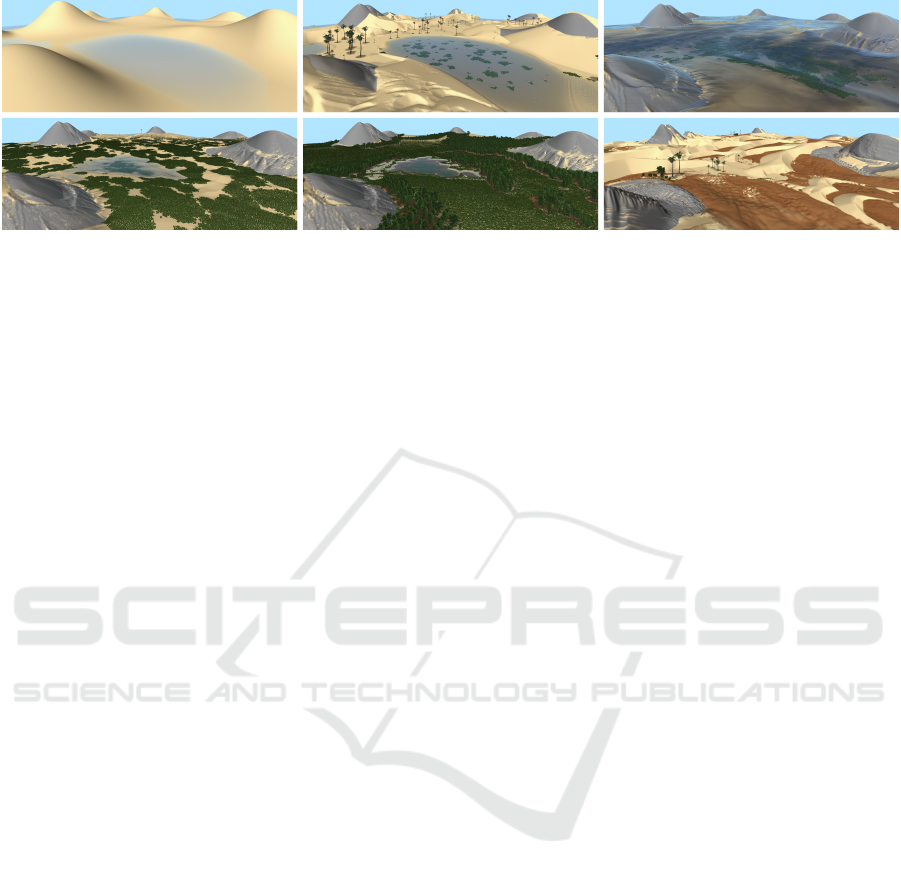
Figure 1: A terrain initialized with low-frequency noise is transformed by a user by changing the rain strength. Initially, rain

is disabled, causing dune formation and aeolian bedrock abrasion. Adapted plants such as palm trees grow in the vicinity of

water sources and seaweed grows under water. The terrain is then ﬂooded with heavy rain, causing strong hydraulic erosion.

Palm trees die in the process and only seaweed can grow, which transforms some sand to soil. Next, rain strength is reduced

signiﬁcantly and most water evaporates. Sufﬁcient moisture prevents saltation and allows for bushes to grow across the entire

scene, which transform sand to soil on a large scale. As soil is generated, trees can begin to grow in the new environment and

start to spread throughout the scene, forming forests. Finally, the user disables rain again. The terrain dries out, causing most

vegetation to die, returning to a desert. The entire process took roughly 15 minutes.

The remainder of this paper is structured as fol-

lows: In Section 2, we introduce relevant related

work. Next, Section 3 introduces our method in de-

tail, followed by our results in Section 4. We con-

clude with Section 5, discussing important directions

for future work and limitations.

2 RELATED WORK

In this section, we will brieﬂy review related work

in computer graphics concerning aeolian erosion, hy-

draulic erosion, vegetation simulation and combined

methods, while focusing on real-time methods.

2.1 Aeolian Erosion

The Desertscape Simulation (Paris et al., 2019) was

the ﬁrst method in computer graphics supporting dune

formation and bedrock abrasion in desert environ-

ments. Barchans, linear dunes, star-shaped dunes and

nabhka dunes are supported and vegetation is con-

sidered via a density map. The simulation is inter-

active, but not real-time. It has since been imple-

mented in real-time on the GPU (Taylor and Keyser,

2023; Nilles et al., 2024a). (Taylor and Keyser, 2023)

added echo dune support and compared their results

with wind tunnel experiments (Tsoar, 1983) and an

accurate ofﬂine method (L

u et al., 2018). In (Nilles

et al., 2024a), the method was further optimized for

the GPU using CUDA and made deterministic. A

new reptation method produces results closer to the

reference method in (L

u et al., 2018). The imple-

mentation has since been expanded with divergence-

free wind ﬁelds and improved reptation (Nilles and

unther, 2024).

2.2 Hydraulic Erosion

Multiple real-time hydraulic erosion methods

emerged since 2007. (Benes, 2007) used the shallow

water equations. Water destroys the terrain and

forms grit (regolith), simulated as a high viscosity

ﬂuid. (Mei et al., 2007) instead use the virtual pipes

method (O’Brien and Hodgins, 1995), paired with

a capacity-based dissolution/deposition model. In

(

St’ava et al., 2008), the virtual pipes method and ero-

sion model from (Mei et al., 2007) are combined with

the shallow water grit simulation from (Benes, 2007).

The method is generalized to multiple different

material layers with varying erosion resistance and

materials age over time. (Kri

stof et al., 2009) used

a 3D smoothed particle hydrodynamics simulation

and perform particle-based erosion on a heightmap

instead. (Hawkins and Ricks, 2023) extended (

St’ava

et al., 2008) with vegetation, modeled as an addi-

tional layer that can die as a result of erosion, forming

another layer which can be transported similar to

sediment. Vegetation reduces the impact of erosion.

However, there is no simulation of vegetation growth

and spread. Recently, (Nilles et al., 2024b) extended

the approach of (Mei et al., 2007) to 3D using

multi-layered heightmaps. Their method is capable

of generating arches, overhangs and limited caves in

real-time.

2.3 Vegetation Simulation

We focus on methods that only consider plant po-

sition, size and type (radius-based methods) instead

of methods simulating detailed growth of individual

plants. An early real-time method considers abiotic

factors such as elevation and slope, which is paired

GRAPP 2025 - 20th International Conference on Computer Graphics Theory and Applications

with noise functions for procedural vegetation place-

ment via an ecosystem probability (Hammes, 2001).

This was extended by (Ch’ng, 2011), which introduce

biotic factors for a more realistic placement of plants.

The Field of Neighborhood (FON) method introduced

in (Berger et al., 2002) uses a circular zone of inﬂu-

ence around each plant, modeling plant competition

that results in growth reduction of neighboring plants.

This was further developed by (Alsweis and Deussen,

2006; Weier et al., 2013), where pregenerated tiles

are used for real-time performance. EcoBrush (Gain

et al., 2017) instead draws interpolated samples from

a database to synthesize a full ecosystem quickly with

interactive control by the user.

A new framework for real-time procedural plant

distribution on large-scale terrains was developed in

(do Nascimento et al., 2018). They consider abiotic

and biotic factors and allow the user to deﬁne plant

types via a set of parameters describing their adapt-

ability, which resembles our approach. Vegetation is

organized in a quadtree, where vegetation only af-

fects plants in layers below it. Moisture is procedu-

rally computed from a wide range of parameters us-

ing inﬂuence curves. Plant overlap is avoided using

distance ﬁelds instead of directly checking plants for

collisions.

Ecoclimates (Pałubicki et al., 2022) is the state-

of-the-art in realism for outdoor landscapes with veg-

etation. The bidirectional relationship between veg-

etation and weather is modeled by combining a 3D

weather simulation, a soil model and a vegetation

model, simulating the entire water cycle. The sim-

ulation is not real-time, but interactive. It is the ﬁrst

method that captures forest edge effects, Foehn and

spatial vegetation patterning.

2.4 Combined Methods

(Cordonnier et al., 2017) combined erosion simu-

lation and vegetation simulation with bidirectional

feedback, which is also the goal of our method. Their

method uses a layered heightmap terrain representa-

tion and an event-based framework. Geomorpholog-

ical events include rainfall, running water, tempera-

ture, lightning, gravity and ﬁre. Ecosystem events

deal with soil moisture, evapotranspiration, illumi-

nation and temperature, which deﬁne the vigor and

stress of plants, resulting in germination, growth or

death and the generation of humus (dark organic

matter in soil). Notably, aeolian erosion or dune

formation are not supported. The event-based na-

ture is ill-suited to the GPU, and their CPU imple-

mentation scales poorly with resolution, requiring

roughly 10× as long when the number of cells is

quadrupled. A simulation step at 1024

resolution re-

quires 38s. Recently, (Hartley et al., 2024) general-

ized erosion on various terrain representations, rang-

ing from heightmaps over multi-layered heightmaps

to 3D voxels, using particles as erosion agents. The

framework can be used for a variety of erosion effects,

such as hydraulic erosion, aeolian erosion and ther-

mal erosion, reproducing the Desertscape Simulation

results from (Paris et al., 2019) to some extent.

3 OUR METHOD

This section will explain our method in detail. The

core components of the simulation are vegetation sim-

ulation, aeolian erosion and hydraulic erosion. A

high-level overview of how these components are

linked together can be found in Figure 2. Aeolian ero-

sion has been adapted from the real-time desertscapes

simulation in (Nilles et al., 2024a) and our implemen-

tation directly extends their code (Nilles and G

unther,

2024). For hydraulic erosion, we have taken ideas

from earlier as well as recent work (Mei et al., 2007;

St’ava et al., 2008; Nilles et al., 2024b). Our vegeta-

tion model is a modiﬁed radius-based model that we

designed speciﬁcally for our erosion simulation.

3.1 Overview

The terrain consists of a 2D grid of N

× N

cells.

Each cell i

i is square with a side length of l

, set to 1m

for all scenes in this paper. The cells form a layered

heightmap, containing bedrock T

, soil T

, sand T

and water T

in that order. Uppercase indicates abso-

lute quantities and lowercase relative quantities, i.e.

W,i

= T

B,i

+ T

e,i

+ T

s,i

+ T

w,i

(1)

is the absolute water height of cell i

i. We deﬁne a veg-

etation height T

, which is relative to the sand height

and overlaps with the water layer. The absolute vege-

tation height is calculated as

V,i

= T

B,i

+ T

e,i

+ T

s,i

+ T

v,i

(2)

and is used for shadow calculation. The 3D position

of the terrain surface is deﬁned as





, T

S,i

, l





(3)

Each cell has a 2D wind velocity w

, calculated

from a high-altitude wind velocity w

, and a 2D water

velocity u

The different components of our simulation inter-

act via an absolute terrain moisture level T

, modeled

up to a depth of 1m. The moisture capacity T

= c

· min(T

e,i

+ T

s,i

, 1), (4)

Oasis: A Real-Time Hydraulic and Aeolian Erosion Simulation with Dynamic Vegetation

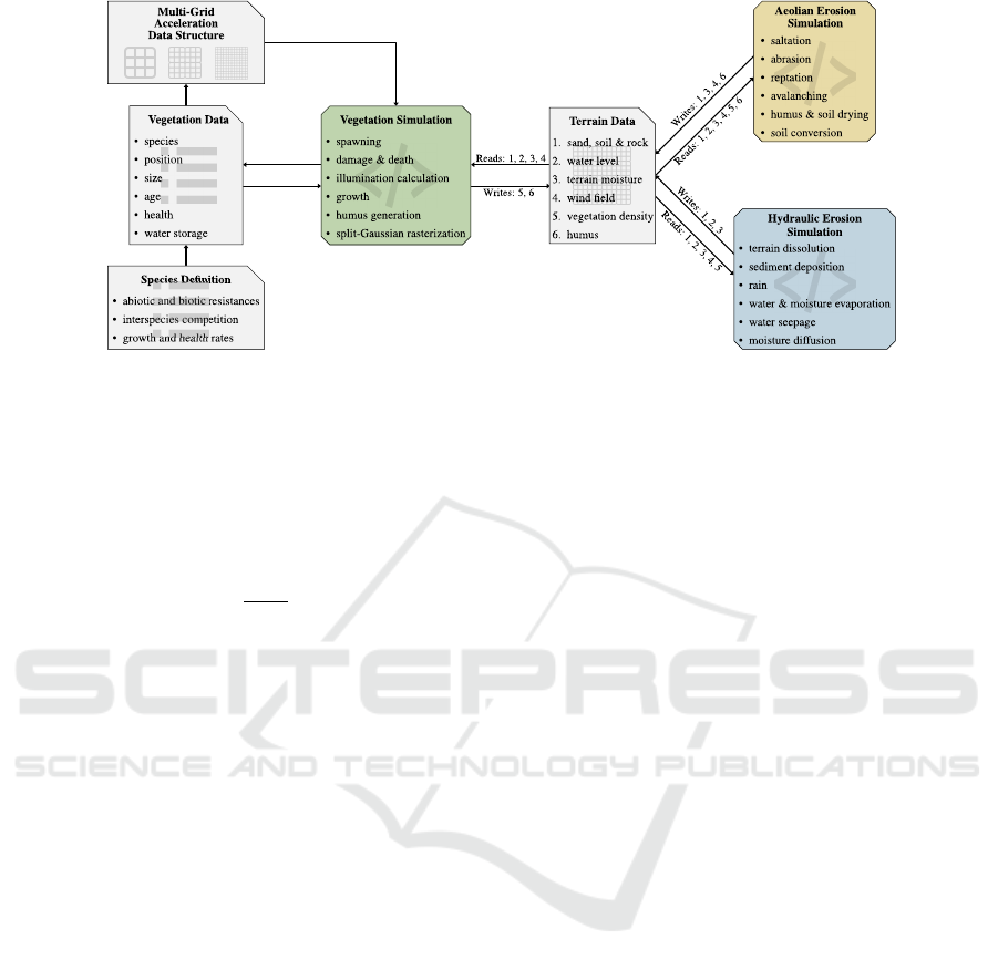
Figure 2: A high-level overview of our method. Terrain data is stored in a 2D grid which serves as the common interface

of vegetation simulation, aeolian erosion and hydraulic erosion, which read and modify the terrain data. This enables bidi-

rectional feedback between the three simulations. The vegetation data is stored as an array, which is only directly read and

modiﬁed by the vegetation simulation. Neighborhood queries for plant competition are accelerated via our multi-grid data

structure. The erosion simulations access the vegetation information via a vegetation density map, which is rasterized from

the actual vegetation using our split-Gaussian model.

where c

is a moisture capacity constant, typically set

to 1. The relative moisture is deﬁned as

m,i

M,i

. (5)

Moisture is used for plant growth and affects aeolian

erosion and the angle of repose of soil and sand.

The aeolian erosion simulation from (Nilles et al.,

2024a) requires a vegetation density T

∈ [0, 1] for

each cell. Instead of using a static vegetation density,

we create the vegetation density map dynamically in

each simulation step, based on the current 3D posi-

tions and sizes of the plants in the scene. It impacts

the angle of repose and aeolian erosion, which we ex-

tend to impact hydraulic erosion and moisture evapo-

ration.

Lastly, aeolian and hydraulic erosion processes

turn soil into sand. We use vegetation to make this

reversible via a humus layer T

h,i

. This layer does not

contribute to the terrain height. It is generated by veg-

etation, decays if there is no moisture present and oth-

erwise slowly transforms sand into soil.

3.2 Vegetation Model

We use a custom radius-based vegetation model tai-

lored to our use case. It is not directly based on pre-

vious work and intentionally simple. More advanced

ideas from related work could be integrated later to

improve our model.

Each plant k has a 3D position V

x,k

, radius V

r,k

health V

h,k

, water storage V

w,k

, age V

a,k

and

species S

. S

is the set of all plants that belong to

species j. The species S

∈ N of a plant determines

how it is adapted to different environmental factors,

how fast it grows, matures and withers, as well as

the maximum radius and how the stem height and

root depth relate to its radius. A competition ma-

trix D

D encodes interspecies competition, where each

entry d

i j

∈ [0, ∞) deﬁnes how much species j reduces

the growth of species i. This can be used to model

species that can coexist easily, compete equally for

resources, or to model an invasive species that com-

pletely dominates another.

Table 1 lists the 26 parameters deﬁning a species

and whether they affect growth, health or the

spawning of new vegetation. We will explain the

most important parameters in detail and refer to

vegetation.cu in the source code for further infor-

mation.

The age of each plant is incremented by ∆t ev-

ery time step and a plant is considered mature if it

has reached the maturity percentage of its maximum

radius in the maturity time. Only mature plants can

reproduce and plants that fail to reach maturity are

removed. Water resistance is used to differentiate

underwater plants from regular plants. A resistance

of 100% indicates a species that only grows under wa-

ter.

The vegetation simulation is structured as follows:

First, vegetation is rasterized into multiple 2D grids

(Section 3.2.1), which bidirectionally links it to the

erosion simulations and is used when spawning new

vegetation (Section 3.2.2). Spawning of new vege-

tation depends on the local and windward density of

each species, as well as compatibility with the envi-

ronment. Next, a two-layered illumination map is cal-

culated using the terrain elevation and rasterized veg-

GRAPP 2025 - 20th International Conference on Computer Graphics Theory and Applications

Table 1: The parameters of a species. A cross marks

whether they affect growth (G), health (H) or spawning of

new vegetation (S). Indirect effects are marked with paren-

thesis.

Parameter G H S

Maximum radius r

max

× × (×)

Growth rate φ

× ×

Position adjust rate φ

(×)

Damage rate φ

Shrink rate φ

(×)

Maturity time × ×

Maturity percentage × ×

Relative stem height h

(×) (×) (×)

Relative root depth h

(×) (×) (×)

Water usage rate φ

× ×

Water capacity w

× ×

Water resistance × × ×

Minimum moisture ×

Maximum moisture × ×

Soil compatibility × ×

Sand compatibility × ×

Maximum stem coverage ×

Minimum root coverage ×

Maximum slope × × ×

Base spawn probability p

Density spawn multiplier p

Wind spawn multiplier p

Humus generation rate φ

Minimum illumination × ×

Maximum illumination × ×

Density separation ρ

etation heights (Section 3.2.3), which is used as an

abiotic growth factor as well as for visualization. We

then calculate the growth of each plant (Section 3.2.4)

depending on the local abiotic and biotic (plant com-

petition) factors. Plants that are unable to grow due

to incompatibility with the environment receive dam-

age, potentially dying, and plants that were unable to

mature in time are culled (Section 3.2.5). Lastly, the

acceleration data structure for neighborhood lookups

is updated (Section 3.2.6).

3.2.1 Rasterizing Vegetation

Our terrain simulation interacts with vegetation in-

directly using the vegetation density map T

. This

needs to be rasterized from the current population of

plants in every simulation step. We describe the den-

sity of a single plant using a split 3D Gaussian, with µ

set to the position of the plant and diagonal covariance

matrix Σ(x

x, k), set to 4V

r,k

horizontally. Vertically,

4(h

s,k

·V

r,k

)

is used for positions above the plant, and

4(h

r,k

· V

r,k

)

below it.

Figure 3: An illustration of our vegetation density model

in 2D for a plant with shallow roots and high stem. The

Gaussian vegetation density is shown in green.

The density of plant k at 3D position x

x is

ρ(x

x, k) = e

−

x−V

x,k

)

Σ(x

x,k)

−1

x−V

x,k

)

. (6)

We further modify this to ensure that the density is 0 if

the distance in the 2D plane is equivalent to the radius,

which is necessary for our acceleration data structure:

ρ(x

x, k) = max



ρ(x

x, k) −

−2

∥x

x − V

x,k

∥

r,k

, 0



. (7)

This is evaluated at the terrain surface x

, which al-

lows us to properly consider height changes in terrain.

If a plant is partially buried under terrain or has its

roots exposed, it will have a lower density. The split

model allows us to describe plants that do not grow

spherically and to specify root depth separately from

height. Figures 3 and 4 illustrate this density model.

The rasterized vegetation density is deﬁned as

V ,i

= min

∑

ρ(x

, k), 1

. (8)

We additionally rasterize the per-species vegetation

density T

V ,i

i, j

by restricting the sum in Equation (8) to

a given species j, which is used when spawning new

plants, alongside a directional per-species vegetation

density which takes the wind direction into account:

W ,i

i, j

∑

k∈S



i, k) ·



1 −

∥x

− V

x,k

∥

max, j



, (9)

i, k) = max



∥w

∥

− V

x,k

∥x

− V

x,k

∥

, 0



. (10)

V ,i

i, j

and T

W ,i

i, j

only consider plants that have

reached maturity, which can reproduce.

Vegetation height is rasterized as

v,i

= max

r,k

· h

s,k

ρ(x

, k)) , (11)

Oasis: A Real-Time Hydraulic and Aeolian Erosion Simulation with Dynamic Vegetation

Figure 4: We visualize the rasterized vegetation density in

green. Damage was disabled, allowing plants to survive if

uprooted or buried. As the terrain changes, vegetation den-

sity adjusts, changing smoothly depending on the distance

to the terrain surface from the plant origin. Plants that are

buried deep or ﬂoating high do not contribute to density.

and the humus map is updated for the next time step

by adding the humus generated by each plant k based

on its humus generation rate φ

h,k

t+∆t

h,i

= T

h,i

+ ∆t ·

∑

h,k

ρ(x

, k). (12)

3.2.2 Spawning Vegetation

In each simulation step, new vegetation can spawn in

any given cell. The species of a spawning plant is

determined using a per species weight

p(i

i, j) = p

b, j

· (1 + p

ρ, j

min(T

V ,i

i, j

, 1)

+ p

W , j

min(T

W ,i

i, j

, 1))

. (13)

In order to avoid vegetation spawning in incompatible

environmental conditions, we reduce the weight of a

species to 0 in those situations. Table 1 shows which

environmental factors we consider. For example, if a

species has a water resistance of 25%, we check the

water level in the cell. If the water level exceeds 25%

of the stem height, the species cannot spawn in this

cell. A species with 100% water resistance is instead

considered to be an underwater plant, which can only

spawn and survive under water.

Furthermore, the density separation parameter ρ

s, j

of a species is used as a threshold. If the per-species

density is larger than this, we set the weight to 0 to

avoid plants spawning too close to each other.

The probability of a vegetation spawn event per

cell and simulation step depends on the sum p

sum

of the per species weights per cell, as well as the total

amount of cells and the time step. As each cell can

only contain a single plant at the same time, we con-

sider

sum

to be the probability of at least one plant

spawning in the cell over the course of 1 second. This

means that the vegetation spawn event has to happen

with probability

spawn

i) = 1 −



1 − min



sum

, 1



∆t

. (14)

If a vegetation spawn event is triggered, the species of

the plant is then selected randomly based on the per

species weights.

Figure 5: Left image: two types of bushes grow in a scene.

One type cannot grow in direct sunlight or strong shadow

and competes with trees, growing only on the shaded side of

a hill and the outer edge of the tree shadow. The other type

has no competition with trees and requires strong shade, so

it grows underneath trees. A closeup is shown in the right

image. The left half of the image is rendered using our vol-

umetric shadow map, the right half has this disabled.

Plants spawn fully healthy with age 0 and no

stored water. Their initial radius is set to 5% of the

maximum possible radius, calculated as

max

i, j) = min



s,i

+ T

e,i

r, j

, r

max, j



. (15)

This considers the root depth of a plant and avoids

plant growth into the bedrock layer.

3.2.3 Illumination

Light is one of the most important growth factors for

plants. Instead of modeling a full day and night cy-

cle with constantly changing shadows and light di-

rection, we model the average illumination through-

out the day. Our approach is motivated from ambient

occlusion, where we introduce a directional bias to-

ward a dominant light direction, usually south. We

compute two illumination values per cell, one for the

ground level and one for the vegetation level. These

can then be interpolated for a given intermediate po-

sition. Figure 5 demonstrates the capabilities of this

model.

Given a cell offset o

o, we calculate the upward tan-

gens angle to the cell at that offset from a given cell i

at the two elevation levels:

α(i

i, o

o) =

∥o

o∥



max(T

V,i

i−o

− T

S,i

, 0)

max(T

V,i

i−o

− T

V,i

, 0)



(16)

and a weight considering light direction l

l and distance

d(i

i, o

o) = −2

max(l

o · l

l), 0)

∥l

· o

o∥

. (17)

Illumination values are then calculated using a 7 × 7

neighborhood by averaging an exponential function:

σ(i

i) =

∑

o∈{−3...3}



d(i

i,o

o)·α

i,o

d(i

i,o

o)·α

i,o



− 1. (18)

GRAPP 2025 - 20th International Conference on Computer Graphics Theory and Applications

The reason for multiplying by 2 and subtracting 1 is

that half of the samples evaluate to 1, so the illumina-

tion value would be in [0.5, 1] without this.

Using Equation (18), we can compute the illumi-

nation at height y via linear interpolation

σ(i

i, y) = (1 − t)σ

i) +tσ

i), where (19)

t =

y − T

S,i

V,i

− T

S,i

. (20)

For underwater plants, we additionally apply an ex-

ponential decay of illumination with water depth.

3.2.4 Vegetation Growth

The rate at which a plant grows is determined by mul-

tiple growth factors g

: Competition with surround-

ing plants g

∈ [0, 1], illumination g

∈ [0, 1], terrain

slope g

∈ [0, 1], water availability g

∈ [1, 2], stand-

ing water g

∈ [0, 1] and ground composition g

∈

[0, 1].

These growth factors are determined based on the

current environment and the species-speciﬁc param-

eters in Table 1. Further effects such as temperature

are left for future work. We use a simpliﬁed model

compared to the piece-wise linear hat-like functions

used for plant response in (Cordonnier et al., 2017)

and other previous work.

For illumination, each species has an interval of

compatible illumination values. The illumination

level is determined by evaluating Equation (19) at the

top of the plant and g

is interpolated based on the

position in the valid interval, where the interval bor-

ders map to 0 and the center of the interval maps to 1.

For example, if the interval is [0.5,1.5], the associ-

ated species starts growing under medium illumina-

tion and growth increases up to the maximum illumi-

nation level of 1. The interval [−0.5, 0.5] describes a

species that only grows in the shade and grows best

at 0 illumination.

The growth factors g

and g

work similarly, the

only difference is that the species determines the right

end of the interval, which maps to no growth, while

ﬂat terrain and absence of standing water lead to the

best growth for these factors. Underwater plants ig-

nore g

Ground composition works differently. It is in-

tended to model nutrients as well as the ability of the

plant’s roots to grow in hard and soft materials. The

sand and soil compatibility of the species are multi-

plied with the percentage of roots covered by that type

of ground and added up. Consequently, the growth

factor g

decreases if the roots are partially exposed

to air. A plant that has 0 compatibility with sand will

thus not grow if the ground entirely consists of sand.

Competition is calculated based on all surround-

ing plants as

c,k

= 1 −

∑

i,i̸=k

· d



min(∥V

x,i

− V

x,k

∥ − (V

r,k

+ V

r,i

), 0)

r,k



. (21)

This roughly approximates how much the radii of two

plants overlap, weighted with the competition rela-

tionship between their associated species. A plant that

spawns in a region with high competition will grow

slowly and potentially not reach maturity.

Lastly, we compute a growth factor for

water availability. Using the volume of the

roots V

r,k

πh

r,k

, stem V

s,k

πh

s,k

r,k

and entire plant V

= V

r,k

s,k

, we determine water

capacity, required water and available ground water

cap

(k) = w

c,k

·V

(22)

req

(k) = ∆t · φ

·V

s,k

(23)

avail

(k) = ∆t · T

M,i

·V

r,k

(24)

If W

avail

< W

req

, the remaining water is taken from the

plants own storage V

, otherwise, the plant can in-

crease its water storage with superﬂuous ground wa-

ter, up to W

cap

. The required water models both water

used by the plant’s cells and water loss due to transpi-

ration. The growth factor g

is 1 if W

req

(k) is satisﬁed

and increases up to 2 if there is an excess of water.

Aside from growth, competition and illumination

also impact the maximum radius of a plant, caus-

ing plants to be smaller in the presence of competi-

tion and bad lightning conditions. The maximum ra-

dius ¯r

max

(k) is further limited by the distance to the

bedrock, similar to Equation (15). It is calculated as

min



x,k

)

− T

B,i

r,k

, g

c,k

· g

I,k

· r

max,k



. (25)

For underwater plants, we additionally consider the

distance to the water surface as a limit.

The plant radius is updated as

t+∆t

r,k

= V

r,k

+ ∆t · φ

∏

i,k

. (26)

If the maximum radius is exceeded, growth is set to 0.

3.2.5 Vegetation Health

The purpose of our vegetation health model is to cull

plants that are no longer able to survive after the envi-

ronmental conditions have changed. A plant receives

damage if its radius is larger than 110% of the current

maximum radius and if the water requirement can-

not be satisﬁed. It is also damaged if illumination is

Oasis: A Real-Time Hydraulic and Aeolian Erosion Simulation with Dynamic Vegetation

outside the compatible interval and if relative ground

moisture or terrain slope exceed a threshold. Lastly,

it is damaged if too much of the plant is underground,

exposed to air or standing water.

Each of these factors results in a damage value d

which is 0 at the border of the allowed range and

grows larger the further the conditions deviate from

allowed values. If any of these damage values ex-

ceeds 0, the plant cannot grow. The health of a plant

is updated using

t+∆t

h,k

= V

h,k

+ ∆t

∏

i,k

− φ

∑

i,k

. (27)

A plant can thus recover its health as it grows. The

maximum health is 1 and if the health reaches 0, the

plant dies and is removed. Plants that fail the maturity

condition have their health set to 0.

Some species are able to shrink, which can be con-

trolled with the shrink rate φ

and only happens if

a plant’s radius exceeds the current maximum by at

least 10%. Similarly, some plants can adjust their po-

sition up or down toward the current ground surface,

which is set via the species parameter φ

. Plants that

can shrink or adjust their position are able to adapt

better to changing environments, avoiding damage.

3.2.6 Acceleration Data Structure

Our vegetation model needs to iterate over all plants

in the scene at various points, which is not possible

in real-time for large plant populations. However, the

inﬂuence of a plant is 0 if it is far enough away. For

the different rasterized quantities, the inﬂuence radius

of a plant is equivalent to its radius V

r,k

. The inﬂu-

ence for the competition calculation g

c,k

depends on

the sum of the radius V

r,k

and the radius of the other

plant.

We thus need a suitable acceleration data structure

for neighborhood lookups. Uniform grids are a good

candidate because they are very efﬁcient to create in

parallel on the GPU. Their resolution has to be chosen

to be optimal for a ﬁxed search radius, but the plants

in our scene have radii varying from 0 to 20m. This

leads to very poor performance in situations where

large and small plants coexist.

Our solution to this problem is to use multiple uni-

form grids at the same time. Each grid covers a dif-

ferent range of radii. We use 4 different scales, with

the respective radii being 0−2.5m, 2.5−5m, 5−10m

and 10 − 20m. The cell size of each uniform grid is

twice the upper bound. Each plant belongs to exactly

one of these grids, which is selected based on its ra-

dius. For rasterization of plant quantities, we only

need to iterate over the plants in 2 × 2 cells of each

uniform grid. Note that our approach is different from

the quadtree used in (do Nascimento et al., 2018), as

we use the data structure solely for a neighborhood

search, whereas the quadtree in the previous work is

used for plant interaction and plants in the same layer

do not interact with each other, only affecting the lay-

ers below them. In our case, all plants interact with

each other.

Competition is more expensive to calculate than

rasterization. When computing the competition of a

small plant, only a few cells in each grid have to be

considered. Large plants have to iterate over a big

area in the higher resolution grids. Our data struc-

ture is thus less optimal for competition calculation.

As there are usually far fewer large plants than small

plants and many more terrain cells than plants in a

scene, rasterization performance was the more impor-

tant factor.

Each uniform grid is allocated densely, so using

multiple grids increases memory. This is negligi-

ble because each successive grid has a signiﬁcantly

smaller resolution. The time required to create mul-

tiple uniform grids is almost equivalent to creating a

single grid in our implementation. In order to achieve

this, we ﬁrst calculate a key for each plant, where the

grid index is encoded in the most signiﬁcant bits and

the least signiﬁcant bits are set to the cell index inside

that grid. We then sort the plants by their keys using

radix sort. A single kernel with one thread per plant

then compares keys of neighboring plants in order to

sparsely ﬁll all uniform grids at once with the respec-

tive start and end indices into the list of plants.

3.3 Aeolian Erosion

Our method directly extends the code of (Nilles et al.,

2024a), so we refer to the original work for exact de-

tails. The object map and echo dunes implementation

proposed by (Taylor and Keyser, 2023) was removed,

as it was not important to our use case. We will give

a brief overview of the method and then highlight the

key changes we made to it.

3.3.1 Overview

The method by (Nilles et al., 2024a) is an enhanced

real-time implementation of (Paris et al., 2019) using

CUDA. It is limited to desertscapes environments and

capable of simulating dune formation and propaga-

tion. Only a bedrock and sand layer are used in the

method and there is no concept of moisture or water.

Vegetation is supported using a static density map that

is unaffected by changes in elevation during the simu-

lation. A simulation step consists of wind ﬁeld calcu-

lation, wind shadow calculation, saltation, sand de-

GRAPP 2025 - 20th International Conference on Computer Graphics Theory and Applications

position/bouncing, abrasion, reptation and avalanch-

ing.

Wind ﬁeld calculation takes a time-varying high

altitude wind direction w

and outputs the 2D wind

ﬁeld w

. This is done by ﬁrst scaling wind strength

with terrain height (venturi effects) and then warp-

ing the wind direction using the gradient of a set of

Gaussian convolutions of the terrain, which was im-

plemented efﬁciently with cuFFT. Since the original

paper in (Nilles et al., 2024a), this has been extended

by creating a divergence-free wind ﬁeld via pressure

projection in the frequency domain, which is sched-

uled to be published after the submission of our pa-

per (Nilles and G

unther, 2024).

Wind shadow calculation traces backward against

the wind direction for each cell and ﬁnds the steep-

est angle up to a maximum distance. This angle de-

termines a wind shadow value in [0, 1]. Angles be-

low 10

◦

cause no shadow, angles above 15

◦

cause full

shadow.

Saltation is the lifting of sand by the wind, as

well as the advection of lifted sand. The amount

of sand that is lifted depends on the vegetation den-

sity T

and wind shadow, which protect from salta-

tion. Advection was originally done using a forward

scheme with atomics, but the divergence-free wind

ﬁeld added later allows for semi-Lagrangian advec-

tion that steps backward in the wind direction while

conserving mass.

Sand deposition and bouncing happen as part of

saltation. After advection, a percentage of lifted sand

is deposited, while the remaining sand is considered

to have bounced on the terrain and remains lifted to be

advected in the next simulation step. The deposition

probability increases with wind shadow and vegeta-

tion density and is also affected by the ground mate-

rial.

Bedrock abrasion to sand happens due to sand that

bounces on bare bedrock. The strength can be set

by the user and is affected by wind speed, vegetation

density and bedrock abrasion resistance.

Reptation describes movements of sand on the

terrain triggered by sand particles colliding with the

ground. (Nilles et al., 2024a) proposed a new method

to support this effect which suffered from some arti-

facts. The current implementation uses an improved

version that implements reptation by adaptively re-

ducing the angle of repose based on the amount of de-

posited and bounced sand (Nilles and G

unther, 2024).

Avalanching refers to the stabilization of sand

slopes toward the angle of repose, set to 33

◦

with no

vegetation and 45

◦

at full vegetation density. This is

implemented using an iterative algorithm. Many iter-

ations are necessary for scenes with strong saltation.

A single avalanching iteration per simulation step is

applied to the bedrock layer, using an angle of 68

◦

3.3.2 Our Changes

As our vegetation model rasterizes the vegetation den-

sity T

needed for aeolian erosion, no further changes

were necessary to support it. We extended the original

method with an additional material layer (soil), which

is fairly straightforward. The soil layer is avalanched

with one iteration per frame, using angles 45

◦

without

vegetation and 68

◦

at full vegetation density.

Similar to bedrock, soil can be abraded due to

saltation, with a separate strength that can be set

by the user. Soil abrasion additionally depends on

moisture by interpolating the strength to 0 as T

m,i

reaches 50%. If moisture is below a threshold m

dry

(2% by default), soil slowly dries out and is trans-

formed into sand:

∆T

e,i

= φ

dry

∆t · (1 − T

V ,i

)

· max(1 −

m,i

dry

, 0) · e

−10·T

s,i

(28)

where φ

dry

= 0.01 is the dry erosion rate. Vegetation

protects from this and dry erosion strength is reduced

by the thickness of the sand above the soil. Equa-

tion (28) is also subtracted from the humus layer T

h,i

Sand can transform back into soil using a combi-

nation of vegetation, humus and moisture, making the

previous processes reversible:

∆T

s,i

= φ

humus

· ∆t · T

V ,i

· T

m,i

, (29)

where φ

humus

= 0.01 is the humus conversion rate.

The humus layer decreases by Equation (29) in the

process.

Lastly, we consider the water layer and moisture

throughout the saltation, deposition and avalanching

process. Sand lifting and abrasion are disabled un-

der water. Additionally, sand can only be lifted if the

relative moisture is below 10%, reaching full strength

at 0%. In order to avoid sand piling up around bodies

of water, the deposition probability is clamped to 1%

in cells with standing water and decreases with mois-

ture, reaching 1% of the original values at 10% rela-

tive moisture. We slightly increase the angle of repose

of soil and sand, reaching a peak at 50% moisture, at

which point the angle of repose drastically decreases

to almost 0

◦

at 100%. This models grit/regolith, caus-

ing the terrain to smooth out under and around water.

3.4 Hydraulic Erosion

We combine several ideas from previous work in our

method (Mei et al., 2007;

St’ava et al., 2008; Nilles

Oasis: A Real-Time Hydraulic and Aeolian Erosion Simulation with Dynamic Vegetation

Figure 6: Strong waves erode the terrain and sediment is washed ashore as sand, forming a beach. After the wave strength is

reduced, the sand that is further inland begins to dry out and is eventually transported away by the wind (last image).

et al., 2024b). The water layer is simulated using

the virtual pipes method, with the GPU implemen-

tation proposed in (Mei et al., 2007). Hydraulic

erosion largely follows the capacity-based dissolu-

tion/deposition model from (Mei et al., 2007), ex-

tended to multiple layers as in (

St’ava et al., 2008).

3.4.1 Overview

Sediment capacity depends on terrain slope and wa-

ter velocity as in previous work. We additionally de-

crease the capacity with increasing water depth, as

proposed in (Nilles et al., 2024b). This is done be-

cause the water velocity calculated in the virtual pipes

model describes the surface, while erosion happens at

the bottom of each water column. Furthermore, the

previous work does not use vegetation. We reduce the

capacity to 50% with increasing vegetation density.

Sand, soil and bedrock can be dissolved into sedi-

ment, which works via user-deﬁned strengths per ma-

terial as in the previous work. The deposition of sed-

iment as sand has been modiﬁed to account for vege-

tation and happens at twice the rate at 100% vegeta-

tion density. In (Mei et al., 2007), semi-Lagrangian

advection was used for sediment due to its sim-

plicity and ease of implementation with GPU tex-

ture fetches. We instead use forward advection with

atomic adds, because the water velocity ﬁeld from the

virtual pipes method is not divergence-free, causing

semi-Lagrangian advection to not conserve mass.

In (

St’ava et al., 2008), the authors additionally

simulate a regolith layer using the shallow water

equations. (Nilles et al., 2024b) simpliﬁed this effect

by modifying the angle of repose with water depth. In

our implementation, this effect is instead controlled

by the terrain moisture as described previously.

3.4.2 Waves

We modify the virtual pipes method such that the

wind ﬁeld from aeolian erosion can interact with it,

generating waves. A sine function is used to create a

time-varying wave strength that depends on the wind:

i) = ∥w

∥ · c

wave

· max(sin(φ

wave

·t), 0) (30)

with wave period φ

wave

and wave strength c

wave

. We

apply exponential decay based on water depth, where

wave strength decreases to 0 with decreasing depth.

This force is then applied to the outﬂow ﬂux in the

virtual pipes method, using the dot product between

outﬂow direction and wind direction.

3.4.3 Rain and Water Sources

The user can specify a minimum and maximum rain

probability p

min

rain

, p

max

rain

, which are interpolated be-

tween based on height, where the maximum is used

at a height h

max

rain

set by the user:

rain

i) = p

min

rain

+ (p

max

rain

− p

min

rain

) ·

W,i

max

rain

. (31)

This probability functions as a threshold for a noise

function η(i

i,t) ∈ [0, 1]. The user can control the time

and space frequencies of this noise function. If the

noise value is less than or equal to the rain probability

in a cell, we add ∆t · φ

rain

to the water level.

A minimum water level can be set for the cells on

the border of the terrain, or all cells in the scene. This

will prevent the water level T

from decreasing below

that point and can be used to create oceans or lakes.

3.4.4 Water Seepage and Moisture Diffusion

Surface water in our simulation slowly seeps into the

ground, turning into ground moisture. Sand and soil

have different seepage rates φ

, φ

. The combined

seepage rate is determined based on the composition

of the terrain up to a depth of 1m as

i) = φ

+ (φ

− φ

) · min(T

s,i

, 1). (32)

This rate is multiplied by 0.02 if the relative ground

moisture is above 50%. If the absolute moisture ex-

ceeds the current capacity T

, the excess moisture

is emitted as surface water. Otherwise, water seeps

into the ground:

∆T

M,i

= min(φ

i) · (T

− T

M,i

), T

w,i

), (33)

which is subtracted from the water layer and added to

the absolute moisture.

We then apply diffusion to the moisture map, us-

ing a single forward iteration of a standard grid-based

diffusion algorithm.

3.4.5 Evaporation

(Mei et al., 2007) implemented evaporation as a per-

centage loss per time step, which behaves inconsistent

GRAPP 2025 - 20th International Conference on Computer Graphics Theory and Applications

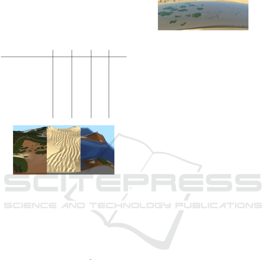
Table 2: Timings in ms of our simulation at 2048

resolu-

tion, with a total of 0.25, 0.5, 1 and 2 million plants. Includ-

ing visualization, the required GPU memory was 1.6GB for

the smallest and 1.8GB for the largest scene. The rows show

timings for the full method and select components. In each

scene, large trees are combined with small bushes that have

no competition and can grow in the shade of trees, which is

particularly challenging for our datastructure.

250k 500k 1m 2m

Full Simulation 16.5 17.5 19.2 23.4

◦ Aeolian 11.7 11.7 11.7 11.6

◦ Sand Aval. 7.6 7.6 7.5 7.4

◦ Hydraulic 2.4 2.4 2.4 2.4

◦ Vegetation 2.4 3.3 5.1 9.3

◦ Data Structure 0.8 1.1 1.6 2.6

◦ Growth 0.7 1.2 2.1 4.6

◦ Raster 0.6 0.8 1.1 1.8

◦ Shadowmap 0.3 0.3 0.3 0.3

Figure 7: From left to right: wetlands, deserts and islands

in an ocean, showcasing possible environments.

with different time steps. We instead use exponential

decay as in (Nilles et al., 2024b):

t+∆t

w,i

= T

w,i

· e

−φ

evap

·∆t

, (34)

where φ

evap

is the user-speciﬁed evaporation rate.

A separate rate can be speciﬁed for ground mois-

ture evaporation, which additionally depends on the

ground material (see Equation (32)) and is reduced

by vegetation:

t+∆t

M,i

= T

M,i

· e

−φ

evap

·φ

i)·∆t·(1−

V ,i

)

. (35)

Evaporation of moisture can only happen if no surface

water is present in a cell.

4 RESULTS

We include two videos that show our results in the

supplementary material, recorded directly during sim-

ulation with a simple real-time renderer.

Our method allows to seamlessly transition be-

tween aeolian erosion with dune formation and hy-

draulic erosion by varying rain, water sources and

evaporation parameters during the simulation, form-

ing a uniﬁed real-time erosion framework, made pos-

sible due to the addition of our ground moisture

Figure 8: Plants protect against hydraulic erosion and en-

courage sediment deposition, demonstrated here with un-

derwater plants. Mounds form around plants, similarly to

nabhka dunes. The right half has vegetation hidden.

model. Using a noise function with a threshold for

rain allows for different parts of the scene to be af-

fected by either type of erosion at the same time. This

can be further controlled by varying the rain proba-

bility with terrain height, allowing the user to restrict

rain to mountains or valleys. We are thus able to sup-

port a wide range of scenes, ranging from completely

dry deserts to wetlands and even islands in an ocean

environment (see Figure 7). Parameters can be ad-

justed on the ﬂy by the user, enabling transformation

of a desert into a lush forest or an underwater environ-

ment and back.

By introducing waves due to wind to the hydraulic

erosion simulation, it is possible to create beaches,

demonstrated in Figure 6. Strong waves erode the ter-

rain and wash sand ashore. If the wave strength is re-

duced, sand that has been washed further inland does

not receive enough moisture from the water anymore,

causing it to be transported away by the wind due to

aeolian erosion if there is no rain.

The dynamic vegetation model proposed by us

improves upon the original static vegetation density

model used for aeolian erosion (Paris et al., 2019).

All shortcomings of the original approach as men-

tioned in (Nilles et al., 2024a) have been addressed,

the vegetation density now appropriately changes as

vegetation is buried or uncovered by sand due to our

3D split-Gaussian model (see Figure 4) which is ras-

terized to a vegetation density in each simulation step.

Additionally, the ideas from (Paris et al., 2019) gen-

eralized well to hydraulic erosion, allowing for the

equivalent of a nabhka dune forming under water

(see Figure 8).

Our vegetation model is coupled bidirectionally to

the erosion simulation. Plants lessen the impact of

erosion and are able to transform landscapes eroded

to just sand back into earthen environments. This in

turn affects vegetation growth, allowing for different

species to grow as the terrain is transformed. The pro-

cess is very ﬂexible, as the user can freely design the

different vegetation species. While there are a total

of 26 parameters that deﬁne a species, the parameters

are intuitive since most of them directly relate to the

conditions they can survive in. To achieve the scene

in Figure 1, a total of 4 species were created. Palm

Oasis: A Real-Time Hydraulic and Aeolian Erosion Simulation with Dynamic Vegetation

trees were conﬁgured to be resilient to being cov-

ered by terrain due to their leaves being placed very

high up, were set to require low amounts of water and

moisture, as well as a preference for sand. This results

in palm trees spawning in a desert environment next

to water sources, forming an Oasis. Seaweed was set

up as an underwater plant and begins to ﬁll the scene

as the terrain is ﬂooded, transforming sand to soil in

the process. After reducing the amount of rain signiﬁ-

cantly, water bodies evaporate again, causing exposed

seaweed to wither. The low amount of rain seeps into

the ground as moisture instead of accumulating as sur-

face water, enabling the growth of bushes across the

entire scene which require more water and moisture.

As the bushes transform sand into soil, trees that re-

quire soil can eventually spawn and displace bushes

due to competition, forming forests as they spread

in the wind direction. Disabling rain causes another

mass extinction event and slowly returns the scene to

a desert as soil dries out and is abraded by aeolian

erosion.

The volumetric illumination model proposed by

us is very efﬁcient to calculate and enables us to fur-

ther diversify the possible plant species. Combined

with the competition model, we can create plants that

only grow in the shade of larger plants or plants that

only grow in the shaded areas of the terrain, but not

in the presence of another species. Together with

the other environmental parameters, it is possible to

have a wide variety of species in the same scene

that each inhabit their own ecological niche (see Fig-

ure 5). We additionally make use of our illumina-

tion model while visualizing the simulation, which

enhances depth perception and replaces traditional

shadow mapping and ambient occlusion techniques

for free.

We evaluate the performance of our simulation on

a RTX 4080 GPU at a terrain resolution of 2048

with

varying number of plants (see Table 2). For each mea-

surement, we imposed an upper limit on the number

of plants, waited until the number of plants reached

this maximum and averaged the next 10,000.00 simu-

lation steps. The scene contains large trees combined

with small bushes that are set to grow in the shade

of larger trees with no competition. This mixture of

densely placed, overlapping plants with high size dif-

ference is particularly demanding, which is why we

chose it to test performance.

The performance of aeolian and hydraulic erosion

is unaffected by the number of plants, with aeolian

erosion requiring about 11.7ms per simulation step.

Hydraulic erosion is very fast at only 2.4ms. Aeo-

lian erosion is more demanding as it involves multiple

fourier transformations, but the main reason is sand

avalanching as in previous work (Nilles et al., 2024a).

We used 50 sand avalanching iterations per simulation

step, requiring around 7.5ms. This many iterations are

only necessary in parts of the scene where dunes are

forming, which was not the case in our scene. An

adaptive approach would thus be very beneﬁcial.

Vegetation computation time grows slower rela-

tive to the number of plants. At two million plants, it

requires 9.3ms per simulation step, bringing the to-

tal method to 23.4ms which is still real-time. The

shadow map creation is independent of the number

of plants and only takes 0.3ms. Vegetation growth is

the most expensive and the only part that grows faster

relative to the number of plants at vegetation count

above one million, requiring 4.6ms for two million

plants, followed by data structure creation with 2.6ms

and vegetation rasterization with 1.8ms. This is ex-

pected as the data structure was optimized for rasteri-

zation. Increasing the number of plants much further

would quickly become limited by vegetation growth

calculation with our current data structure, indicating

that even more plants are possible in real-time if this

is improved.

5 CONCLUSION AND FUTURE

WORK

In conclusion, we successfully integrated aeolian ero-

sion, hydraulic erosion, and vegetation simulation

into a single method capable of real-time performance

at resolutions of 2048

with two million plants, made

possible by our acceleration data structure. The dif-

ferent components were tied together by adding a

ground moisture level and our split-Gaussian vege-

tation density rasterization. Our vegetation model

supports multiple plant species, including underwa-

ter vegetation, which can be conﬁgured alongside

other parameters like rain and water sources. Each

species is deﬁned by simple parameters based on en-

vironmental compatibility, paired with a basic volu-

metric illumination calculation. It is possible to in-

teractively transform between entirely different envi-

ronments, such as deserts, underwater landscapes and

lush forests, while observing changes in real-time.

For future work, we would like to further improve

the vegetation data structure to allow for even larger

numbers of plants in real-time. Additionally, the sand

avalanching step from aeolian erosion still has a high

cost, as in the previous work. Performance could

be increased by adaptively reducing the number of

avalanching steps used, as only dry deserts require

many iterations. Alternatively, it would be worth in-

vestigating a machine learning solution to avalanch-

GRAPP 2025 - 20th International Conference on Computer Graphics Theory and Applications

ing. A neural network could be trained by using

the current avalanching implementation to produce a

ground truth.

We have not yet incorporated temperature into our

simulation, which is another important factor for veg-

etation growth. In order to support the full range

of real-world temperatures, we would like to com-

bine this with snow and ice simulations, potentially

accounting for thermal erosion. In particular, the

aeolian erosion framework seems well-suited to be

adapted for snow dune simulation. Using real-world

elevation and weather data or alternatively, a full

weather simulation are other avenues worth explor-

ing. In a similar manner, further weather effects such

as lightning strikes, as well as forest ﬁres as imple-

mented in (Cordonnier et al., 2017) are not yet con-

sidered.

Another limitation of our model is the high num-

ber of parameters, which make interaction more com-

plex for an artist in the current state. As pointed out

by a reviewer, we think that further work should iden-

tify meaningful presets and organize parameters into

main parameters as well as less important ones for

ﬁne-tuning. Another possibility would be developing

a set of more intuitive meta-parameters that control

the current parameters behind the scenes.

Lastly, there is a wide array of research available

with more realistic vegetation models. As our ex-

pertise is in erosion simulations and our goal was to

combine multiple different simulations into a single

real-time implementation, we chose to leave this ad-

ditional complexity out and developed our own sim-

ple method, allowing us to freely design the vegeta-

tion model to suit the needs of the erosion simulation.

Incorporating the state of the art in vegetation simula-

tions is thus left for future work.

ACKNOWLEDGEMENTS

The textures and meshes used for trees, bushes and

seaweed are from Sketchfab users (evan4129, 2024;

OwenCalingasan, 2024) and licensed as CC BY

4.0 (Creative Commons, 2024).

REFERENCES

Alsweis, M. and Deussen, O. (2006). Wang-tiles for the

simulation and visualization of plant competition. In

Nishita, T., Peng, Q., and Seidel, H.-P., editors, Ad-

vances in Computer Graphics, pages 1–11, Berlin,

Heidelberg. Springer Berlin Heidelberg.

Benes, B. (2007). Real-Time Erosion Using Shallow Water

Simulation. In Dingliana, J. and Ganovelli, F., editors,

Workshop in Virtual Reality Interactions and Physi-

cal Simulation ”VRIPHYS” (2007). The Eurographics

Association.

Berger, U., Hildenbrandt, H., and Grimm, V. (2002). To-

wards a standard for the individual-based modeling

of plant populations: self-thinning and the ﬁeld-of-

neighborhood approach. Natural Resource Modeling,

15(1):39–54.

Ch’ng, E. (2011). Realistic placement of plants for virtual

environments. IEEE Computer Graphics and Appli-

cations, 31(4):66–77.

Cordonnier, G., Galin, E., Gain, J., Benes, B., Gu

erin, E.,

Peytavie, A., and Cani, M.-P. (2017). Authoring land-

scapes by combining ecosystem and terrain erosion

simulation. ACM Trans. Graph., 36(4).

Creative Commons (2024). CC BY 4.0 Attribution 4.0 In-

ternational. https://creativecommons.org/licenses/by/

4.0/.

do Nascimento, B. T., Franzin, F. P., and Pozzer, C. T.

(2018). Gpu-based real-time procedural distribution

of vegetation on large-scale virtual terrains. In 2018

17th Brazilian Symposium on Computer Games and

Digital Entertainment (SBGames), pages 157–15709.

evan4129 (2024). LOD/Billboard Summer Trees Pack,

Trees and bush Pack LOWPOLY, Palm Tree Pack

LOWPOLY. https://sketchfab.com/evan4129.

Gain, J., Long, H., Cordonnier, G., and Cani, M.-P. (2017).

Ecobrush: Interactive control of visually consistent

large-scale ecosystems. Computer Graphics Forum,

36(2):63–73.

Hammes, J. (2001). Modeling of ecosystems as a data

source for real-time terrain rendering. In Westort,

C. Y., editor, Digital Earth Moving, pages 98–111,

Berlin, Heidelberg. Springer Berlin Heidelberg.

Hartley, M., Mellado, N., Fiorio, C., and Faraj, N. (2024).

Flexible terrain erosion. The Visual Computer.

Hawkins, B. and Ricks, B. (2023). Improving virtual

pipes model of hydraulic and thermal erosion with

vegetation considerations. The Visual Computer,

39(7):2835–2846.

Kri

stof, P., Bene

s, B., K

riv

anek, J., and

St’ava, O. (2009).

Hydraulic erosion using smoothed particle hydrody-

namics. Computer Graphics Forum, 28(2):219–228.

u, P., Dong, Z., and Rozier, O. (2018). The Combined

Effect of Sediment Availability and Wind Regime on

the Morphology of Aeolian Sand Dunes. Journal of

Geophysical Research: Earth Surface, 123(11):2878–

2886.

Mei, X., Decaudin, P., and Hu, B.-G. (2007). Fast Hydraulic

Erosion Simulation and Visualization on GPU. In 15th

Paciﬁc Conference on Computer Graphics and Appli-

cations (PG’07), pages 47–56.

Nilles, A. M. and G

unther, L. (2024). CUDA

Dune Simulation. https://github.com/Clocktown/

CUDA-Dune-Simulation.

Nilles, A. M. and G

unther, L. (2025). Oasis. https://github.

com/Clocktown/Oasis/tree/GRAPP2025.

Nilles, A. M., G

unther, L., and M

uller, S. (2024a). Real-

Time Desertscapes Simulation with CUDA. In Pro-

ceedings of the 19th International Joint Conference

Oasis: A Real-Time Hydraulic and Aeolian Erosion Simulation with Dynamic Vegetation

on Computer Vision, Imaging and Computer Graphics

Theory and Applications - Volume 1: GRAPP, pages

34–45. INSTICC, SciTePress.

Nilles, A. M., G

unther, L., Wagner, T., and M

uller, S.

(2024b). 3D Real-Time Hydraulic Erosion Simula-

tion using Multi-Layered Heightmaps. In Linsen, L.

and Thies, J., editors, Vision, Modeling, and Visual-

ization. The Eurographics Association.

O’Brien, J. and Hodgins, J. (1995). Dynamic simulation

of splashing ﬂuids. In Proceedings Computer Anima-

tion’95, pages 198–205.

OwenCalingasan (2024). Seaweed. https://sketchfab.com/

OwenCalingasan.

Pałubicki, W., Makowski, M., Gajda, W., H

adrich, T.,

Michels, D. L., and Pirk, S. (2022). Ecoclimates:

climate-response modeling of vegetation. ACM Trans.

Graph., 41(4).

Paris, A., Peytavie, A., Gu

erin, E., Argudo, O., and Galin,

E. (2019). Desertscape Simulation. Computer Graph-

ics Forum, 38(7):47–55.

Taylor, B. and Keyser, J. (2023). Real-Time Sand Dune

Simulation. Proc. ACM Comput. Graph. Interact.

Tech., 6(1).

Tsoar, H. (1983). Wind Tunnel Modeling of Echo and

Climbing Dunes. In Brookﬁeld, M. and Ahlbrandt, T.,

editors, Eolian Sediments and Processes, volume 38

of Developments in Sedimentology, pages 247–259.

Elsevier.

St’ava, O., Bene

s, B., Brisbin, M., and K

riv

anek, J.

(2008). Interactive terrain modeling using hydraulic

erosion. In Proceedings of the 2008 ACM SIG-

GRAPH/Eurographics Symposium on Computer An-

imation, SCA ’08, page 201–210, Goslar, DEU. Eu-

rographics Association.

Weier, M., Hinkenjann, A., Demme, G., and Slusallek, P.

(2013). Generating and rendering large scale tiled

plant populations. 10(1).

GRAPP 2025 - 20th International Conference on Computer Graphics Theory and Applications