Adaptable Distributed Vision System for Robot Manipulation Tasks

Marko Pavlic

and Darius Burschka

Machine Vision and Perception Group, Chair of Robotics, Artiﬁcial Intelligence and Real-time Systems,

Technical University of Munich, Munich, Germany

{marko.pavlic, burschka}@tum.de

Keywords:

Vision for Robotics, Scene Understanding, 3D Reconstruction, Features Extraction, Optical Flow.

Abstract:

Existing robotic manipulation systems use stationary depth cameras to observe the workspace, but they are

limited by their ﬁxed ﬁeld of view (FOV), workspace coverage, and depth accuracy. This also limits the

performance of robot manipulation tasks, especially in occluded workspace areas or highly cluttered envi-

ronments where a single view is insufﬁcient. We propose an adaptable distributed vision system for better

scene understanding. The system integrates a global RGB-D camera connected to a powerful computer and

a monocular camera mounted on an embedded system at the robot’s end-effector. The monocular camera fa-

cilitates the exploration and 3D reconstruction of new workspace areas. This conﬁguration provides enhanced

ﬂexibility, featuring a dynamic FOV and an extended depth range achievable through the adjustable base

length, controlled by the robot’s movements. The reconstruction process can be distributed between the two

processing units as needed, allowing for ﬂexibility in system conﬁguration. This work evaluates various con-

ﬁgurations regarding reconstruction accuracy, speed, and latency. The results demonstrate that the proposed

system achieves precise 3D reconstruction while providing signiﬁcant advantages for robotic manipulation

tasks.

1 INTRODUCTION

Scene understanding is critical for a robot manipula-

tor to interact successfully with his surroundings. The

robot needs to know what objects are in his workspace

and their precise location in the scene. Existing de-

ployed robotic manipulators often have limited per-

ception of the surroundings. Usually, a single static

depth camera is used to observe the robot workspace.

Such a setup has a ﬁxed ﬁeld of view (FOV) and

therefore suffers from occlusion. The robot arm or

large objects can cause these occlusions. Further-

more, the accuracy of the depth data decreases with

the distance to the camera, which means the details of

small objects are lost. This leads to inaccuracies in

object recognition, especially in object pose estima-

tion, which considerably limits precise manipulation.

The camera must be brought close to the scene to bet-

ter understand it. Mounting a camera directly on the

end-effector allows the robot to explore its workspace

more ﬂexibly and dynamically. Integrating a pro-

cessing unit at the end-effector eliminates the need

to transmit entire image data to a remote processing

unit, thereby improving efﬁciency. This processing

https://orcid.org/0000-0002-2325-2951

https://orcid.org/0000-0002-9866-0343

ROI

Feature

Extraction

Feature

Matching

Recover

Camera

Pose

SfM

Sparse

Point

Cloud

Accuracy

Robot

State

Embedded

System

Central

System

Stereo

Dense

Point

Cloud

Feature

Manager

Kalman

Filter

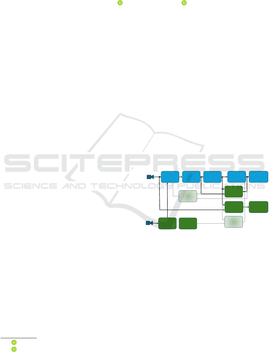
Figure 1: Software architecture of the Distributed Vision

System. Shared modules are shown in blue, whereas green

modules run fully on the central processing unit.

unit must be appropriately designed to match the pay-

load capacity of the robot arm.

This paper introduces a system capable of explor-

ing and reconstructing occluded workspace regions

using an eye-in-hand camera integrated with an em-

bedded system mounted directly on the end-effector.

The embedded system communicates with a more

powerful central processing unit via Ethernet. The

3D reconstruction of a static scene is typically com-

posed of four stages: feature extraction, feature map-

ping, camera pose estimation, and triangulation from

correspondences. These stages are illustrated in the

blue boxes in Figure 1. The proposed system en-

ables ﬂexible distribution of these tasks between the

Pavlic, M. and Burschka, D.

Adaptable Distributed Vision System for Robot Manipulation Tasks.

DOI: 10.5220/0013115600003912

Paper published under CC license (CC BY-NC-ND 4.0)

In Proceedings of the 20th International Joint Conference on Computer Vision, Imaging and Computer Graphics Theory and Applications (VISIGRAPP 2025) - Volume 2: VISAPP, pages

651-658

ISBN: 978-989-758-728-3; ISSN: 2184-4321

651

two computing units based on reconstruction require-

ments such as accuracy, speed, and latency. This pa-

per conducts a detailed analysis of various distribu-

tions of the reconstruction process between the two

processing units, examining the advantages and dis-

advantages of each conﬁguration.

Our contribution is an adaptive distributed vi-

sion system for robot manipulators with the following

properties:

1. Sparse and dense 3D reconstruction of initially in-

visible workplace areas with a monocular camera

mounted on an end-effector

2. Workload sharing between a powerful worksta-

tion and a less powerful embedded system, de-

pending on the application

3. Adaptable stereo system to overcome the limita-

tions of conventional stereo systems

The rest of the paper is organized as follows: Sec-

tion 2 discusses related work before we present the

physical architecture in Section 3 and the used meth-

ods in Section 4 followed by the experiments and re-

sults in Section 5. Finally, Section 6 concludes with a

summary and outlook on future directions.

2 RELATED WORK

3D reconstruction has made enormous progress in re-

cent years (McCormac et al., 2018), (Sch

onberger and

Frahm, 2016), (Hirschmuller, 2005), but existing de-

ployed robot manipulators still have limited percep-

tion of their surrounding (Lin et al., 2021). Most

robotic systems like in works of (Kappler et al., 2017),

(Murali et al., 2019) or (Shahzad et al., 2020) use

RGB-D information from a single view for robotic

manipulation tasks. Due to the ﬁxed FOV, these sys-

tems suffer from occlusions and only partially recon-

struct the workspace. In the work of (Zhang et al.,

2023), they overcome the limitations from a single

view by using multiple cameras to capture an ob-

ject from different perspectives. The working area is

signiﬁcantly restricted with this setup. In the work

of (Lin et al., 2021), a system was designed for en-

hanced scene awareness in robotic manipulation, uti-

lizing RGB images captured from a monocular cam-

era mounted on a robotic arm. The system aims to

generate a multi-level representation of the environ-

ment that includes a point cloud for obstacle avoid-

ance, rough poses of unknown objects based on prim-

itive shapes, and full 6-DoF poses of known objects.

This work shows similar ideas to ours, but they use

Deep-Learning-based approaches to create 3D recon-

structions and ﬁt objects’ shapes. The work of (Hagi-

wara and Yamazaki, 2019) also uses an eye-in-hand

setup, describing an approach for a very speciﬁc ma-

nipulation task. YOLO (Redmon et al., 2015) was

trained to detect valves, and by assumption about the

valve diameter, the localization in space was calcu-

lated from the bounding box returned by YOLO. The

study in (Arruda et al., 2016) aims to improve robotic

grasping reliability through active vision strategies,

particularly for unfamiliar objects. It identiﬁes two

primary failure modes: collisions with unmodeled

objects and insufﬁcient object reconstruction, which

affect grasp stability. The researchers pursue the

same goal of fully reconstructing the scene, especially

for unknown objects. However, stereo cameras are

bulkier, heavier, and less adaptable due to their ﬁxed

conﬁguration, resulting in a constrained depth range

and accuracy. Despite advancements in scene un-

derstanding for robotic manipulation, there remains a

signiﬁcant need for a ﬂexible active perception system

capable of efﬁciently acquiring relevant information.

3 SYSTEM ARCHITECTURE

The software architecture of the proposed distributed

system is illustrated in Figure 1. The system con-

sists of various conﬁgurable modules for sparse and

dense 3D reconstruction of the robot workplace. The

blue modules are implemented across both process-

ing units (embedded and central system), enabling

a ﬂexible distribution of the sparse 3D reconstruc-

tion pipeline. Depending on the computational ca-

pabilities of the embedded system, speciﬁc prepro-

cessing tasks can be performed locally, reducing the

amount of data that must be transmitted. In some

cases, the embedded system can handle the complete

reconstruction process, contingent upon the recon-

struction requirements. Additionally, this work in-

corporates a module for evaluating key performance

metrics, including reconstruction accuracy and frame

rate, across various system conﬁgurations. Green

modules in Figure 1 are computationally expensive

and must run on the more powerful central system.

Slightly transparent modules show ideas for future

work.

4 MODULES

4.1 Feature Extraction and Matching

Depending on the requirements for speed, accuracy,

and robustness of transformations, our module of-

fers different feature detectors to choose from. One

simple and very efﬁcient one is the FAST (Features

VISAPP 2025 - 20th International Conference on Computer Vision Theory and Applications

652

from Accelerated Segment Test) (Rosten and Drum-

mond, 2006) feature detector. Still, it is not scale-

invariant and struggles with signiﬁcant rotations and

scale changes. Next, we have SIFT (Scale-Invariant

Feature Transform) (Lowe, 2004) features, which are

invariant to scale and rotation, partly invariant to

illumination, and robust to limited afﬁne transfor-

mation. The algorithm ensures high distinctiveness

and produces many features but is computationally

expensive. Alternatively, SURF (Speeded Up Ro-

bust Features) (Bay et al., 2006) or ORB (Oriented

FAST and Rotated BRIEF) (Rublee et al., 2011) fea-

tures can be chosen, which are computationally faster

compared to SIFT but still offer reasonable accu-

racy. Another widespread feature detection and de-

scription algorithm is AKAZE (Accerlerated-KAZE)

(Fern

andez Alcantarilla, 2013), which balances speed

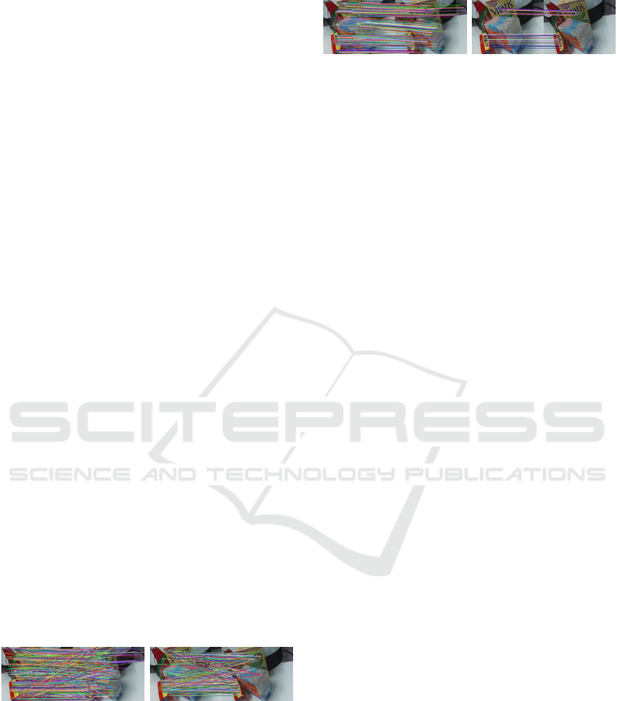
and accuracy well. Figure 2 shows an example of the

unﬁltered feature matching between two images using

(a) SIFT and (b) ORB.

Good feature matching is critical when using im-

ages for 3D reconstruction. The matching results will

directly determine whether the camera pose estima-

tion is reliable. Some standard methods for elim-

inating mismatches are the threshold and nearest-

neighbor distance ratios. The former must set a cer-

tain threshold to eliminate wrong matches, which re-

lies on manual adjustment. The latter calculates the

ratio of the closest distance to the next closest dis-

tance around the matching point. If it is less than

the ratio threshold, the match is retained. Otherwise,

it needs to be ﬁltered. In addition, when determin-

ing the essential matrix E, which is described in the

next chapter, some matches are ﬁltered out during

the RANSAC optimization. Figure 3 shows the ﬁl-

tered matching results with correctly assigned feature

points between the images. It is easy to see here that

the very robust descriptors of the SIFT algorithm re-

tain many matches, which is helpful for an accurate

camera pose estimation. The speed advantage of the

ORB algorithm will be shown later in the results.

(a) SIFT (b) ORB

Figure 2: The matching of image features using (a) SIFT

and (b) ORB.

4.2 Camera Pose Recovery

After ﬁnding the corresponding features in two im-

ages, the epipolar constraint can be used to recover

the camera pose. Image points can be represented as

(a) SIFT (b) ORB

Figure 3: The ﬁltered matching results using (a) SIFT and

(b) ORB.

homogeneous three-dimensional vectors p and p

′

the ﬁrst and second view, respectively. The homoge-

neous four-dimensional vector P represents the corre-

sponding world point. The image projection is given

p ∼ K



R t



P (1)

where K is a 3 × 3 camera calibration matrix, R is a

rotation matrix and t a translation vector. The ∼ de-

notes equality up to scale. Let the camera matrices for

the two views be A = K

[I | 0] and A

′

= K

[R | t].

Let [t]

denote the skew-symmetric matrix so that

[t]

x = t × x for all vectors x.

The fundamental matrix F is then deﬁned as

F = K

−T

[t]

−1

(2)

which encodes the well-known epipolar constraint:

′T

Fp = 0. (3)

For calibrated cameras, the matrices K

and K

are

known and the matrix E = [t]

R is called the essential

matrix. A common algorithm to solve for the camera

pose is decomposing the essential matrix using SVD

(Nister, 2004). Although the rotation matrix is cor-

rectly determined, only the translation’s direction is

computed. The correct scale s for the translation vec-

tor is computed with the information on the robot’s

state at every image capture and gives the corrected

translation vector T = st.

4.3 Sparse 3D Reconstruction

With the camera pose computed in the previous step,

the point in space for each image point correspon-

dence p, p

′

can be computed up to scale using (1).

Since there are usually errors in the measured image

points, there will not be a point P which exactly satis-

ﬁes p = AP and p

′

= A

′

P. The aim is to ﬁnd an esti-

mate

P which minimizes the reprojection error (Hart-

ley and Zisserman, 2004). A sparse point cloud of the

observed scene is the result.

4.4 Dense 3D Reconstruction

For a dense 3D reconstruction, the depth is estimated

for nearly every pixel of the image, which is computa-

tionally intensive but gives a detailed view of the en-

vironment. A widely used vision algorithm for dense

Adaptable Distributed Vision System for Robot Manipulation Tasks

653

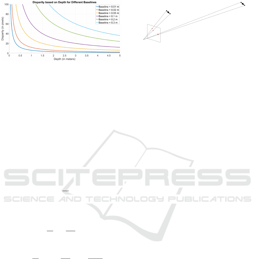
Figure 4: Disparity-Depth graphs for a classical stereo sys-

tem for different baselines.

depth estimation is Semi-Global Matching (SGM)

(Hirschmuller, 2005), which computes a dense dis-

parity map between image pairs. SGM allows for a

good trade-off between accuracy and computational

efﬁciency, making it popular in robotics. It operates

on minimizing a cost function that accounts for pixel-

wise matching costs and a smoothness constraint. The

smoothness constraint helps to maintain coherence in

disparity maps, especially at object boundaries, where

abrupt changes occur. The key advantage of SGM is

its ability to produce high-quality disparity maps with

subpixel accuracy, making it suitable for detailed 3D

reconstructions.

The depth z (in m) can be estimated from the dis-

parity d (in pixels) by stereo triangulation without

systematic and random errors:

z =

b f

(4)

where b is the stereo baseline (in m), and f is the focal

length (in pixels). To understand how depth resolution

changes with disparity, we compute the derivative of

depth z with respect to disparity d:

= −

f · b

(5)

For a small change ∆d in disparity, the corresponding

change in depth ∆z is:

∆z ≈

· ∆d = −

f · b

· ∆d =

· ∆d

(6)

As a result, the depth resolution diminishes with the

square of the depth (Wang and Shih, 2021), as illus-

trated in Figure 4. A small change in disparity ∆d

leads to a signiﬁcant change in depth ∆z, indicating

that objects farther from the sensor have lower depth

resolution. Our sensor system allows for control of

both the base width and the distance to the scene

through robot movement, ensuring that the system op-

erates within the optimal sensor range.

4.5 System Evaluation

The pipeline from image acquisition to sparse point

cloud generation, shown in Figure 1, can be arbitrarily

Figure 5: The same 3D error corresponds to different 2D

errors depending on the distance of the point to the camera

(Burschka and Mair, 2008).

divided between the central and embedded systems.

The division of the reconstruction process depends on

the hardware and the system’s requirements for accu-

racy, speed, and latency of reconstruction. Thus, care-

ful consideration is needed to determine the optimal

distribution of tasks between the central and embed-

ded systems. Additionally, we have integrated a crit-

ical software component that enables automatic sys-

tem performance evaluation.

On the one hand, the runtimes of the individual

process steps and the data transfer time between the

two processing units are measured. Remote proce-

dure calls (RPC) are used for communication, where

the central system requests a procedure from the em-

bedded system and waits for the response. The maxi-

mum achievable frame rate, used as the key parameter

for speed, is determined by the reciprocal of the com-

bined processing time and data transfer time.

On the other hand, the estimated camera pose is

decisive for the quality of the reconstruction. The

2D reprojection error e

is usually used for accuracy

evaluation. It is calculated as the root mean square

(RMS) error between the actual 2D points p

i, j

and the

projected 2D points

i, j

. But as seen in Figure 5, a

3D error can have different 2D errors depending on

the distance of the point to the camera. For a better

evaluation of the accuracy of the presented system,

the 3D reprojection error is calculated.

A 3D point P

i−1, j

can be reprojected from image

i − 1 to image i using the estimated rotation R and

translation T as

i, j

= RP

i−1, j

+ T. (7)

According to Figure 6, any point P

in the world

can be written as a product of its direction n

and the

radial distance λ

. Therefore, (7) can also be written

i, j

. (8)

For the corresponding 2D point p

i, j

= (u

i, j

, v

i, j

)

the direction can be calculated by

VISAPP 2025 - 20th International Conference on Computer Vision Theory and Applications

654

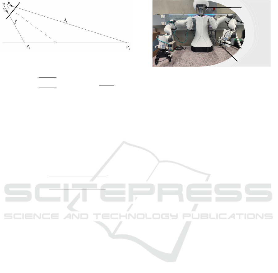
Figure 6: Radial distance λ

and direction n

to the imaged

point (Burschka and Mair, 2008).

i, j







i, j

−C

)

i, j

−C

)







⇒ n

i, j

||k

i, j

(9)

The radial distance λ

i, j

is assumed to be the same

as for the projected point, and so the actual 3D point

i, j

can be calculated as

i, j

. (10)

Similar to the 2D projection error, the 3D repro-

jection error e

is calculated as the root mean square

(RMS) error between the actual 3D points P

i j

and the

projected 3D points

i j

∑

i=1

∑

j=1



i j

−

i j



∑

i=1

(11)

where P

i j

is the j-th 3D point in the i-th image and

i j

is the corresponding projected 3D point. M is the

total number of images and N

is the number of points

in the i-th image.

This evaluation allows for selecting the best possi-

ble system workload for the respective hardware and

application. This is particularly important if the sys-

tem is used as a sensor input for controlling the robot.

In this case, latencies should ideally be zero.

5 EXPERIMENTS AND RESULTS

As shown in Figure 7, the hardware utilized in

the experiments consists of several key components.

The central unit is a powerful workstation with an

NVIDIA GeForce GTX4080 GPU. The head camera

is an industrial RGB-D camera connected to the cen-

tral unit. The robot arm is a 7-DOF Franka Panda

robotic manipulator responsible for the physical ma-

nipulation tasks. The embedded system is a Rasp-

berry Pi 4B, mounted on the robot’s end-effector,

which supports local processing. An eye-in-hand

monocular camera is connected to the Raspberry Pi

4B, providing visual data from the end-effector’s per-

spective. Communication between the central and

RGB-D Head

Camera

Franka

Manipulator

Embedded System

Raspberry Pi 4B

Monocular

Camera

Figure 7: A dual arm manipulation platform with two

Franka Emika Panda Robots and the distributed vision sys-

tem proposed in this paper.

embedded system is established through RPC, with

the brain assuming the leading role in the system’s

operations.

5.1 System Performance

This subsection analyzes the effects of splitting the

sparse reconstruction process between the central

unit and the embedded system on reconstruction

speed, accuracy, and latency. A data set of 50 simple

scenes (single objects) and 50 cluttered scenes (many

objects), each with 25 images from different perspec-

tives, was created for the experiments. Table 1 shows

the result of our experiment. The columns represent

four system conﬁgurations that are examined:

1. Conﬁguration 1: The embedded system sends

whole images to the main processing unit, and the

reconstruction runs fully on the central unit.

2. Conﬁguration 2: The embedded system per-

forms the feature detection and transfers feature

points with their corresponding descriptor, and the

matching, pose estimation, and triangulation runs

on the central unit.

3. Conﬁguration 3: The embedded system runs

feature detection and matching and transfers the

matched feature points with their descriptor to the

central unit to perform pose estimation and trian-

gulation.

4. Conﬁguration 4: The whole 3D reconstruction

runs on the embedded system.

The parameters detect, match, and SfM show the

total duration of the respective reconstruction step for

all 50 data sets with 25 images each. The parameter

data transfer shows the duration needed to communi-

cate between the central unit and the embedded sys-

tem. The maximum achievable frame rate is shown as

FPS, and the 3D reprojection error is shown as e

The different system conﬁgurations were also run

for different feature detectors. Comparing the indi-

Adaptable Distributed Vision System for Robot Manipulation Tasks

655

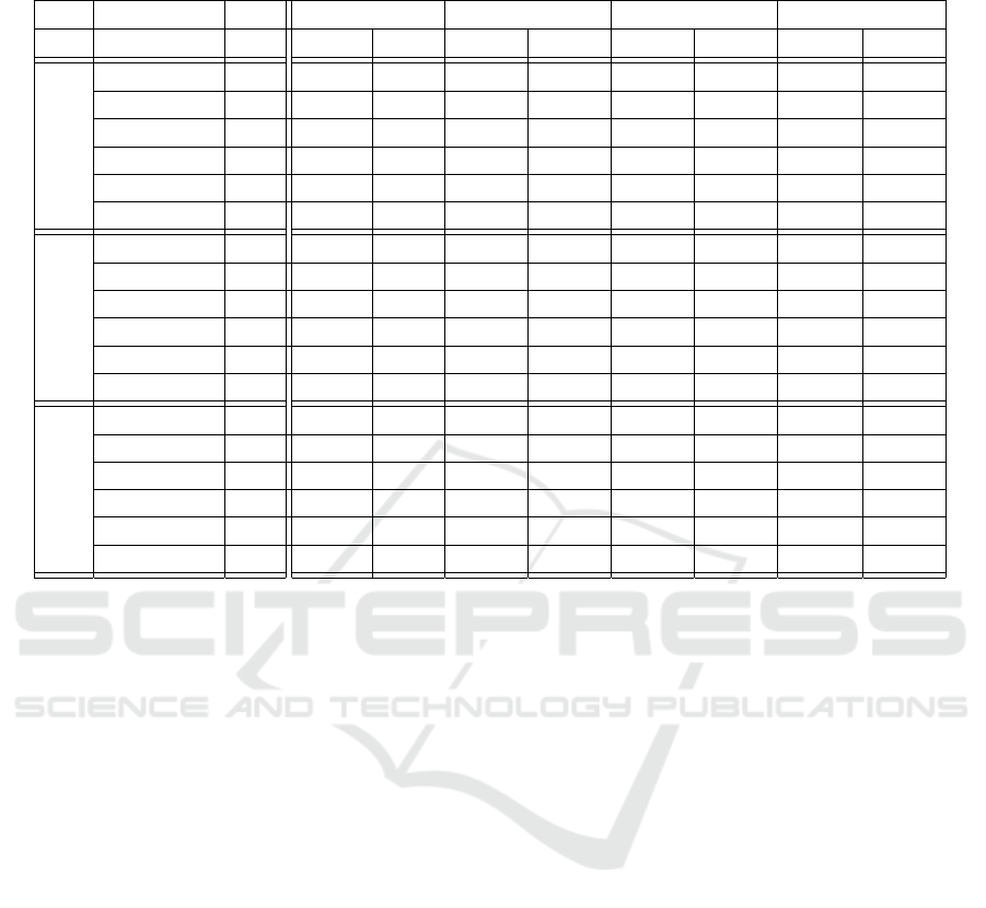
Table 1: Estimated frame rate and reprojection error with different feature detectors and conﬁgurations of the distributed

vision system.

Det. Parameter Unit Conﬁg. 1 Conﬁg. 2 Conﬁg. 3 Conﬁg. 4

simple clutt. simple clutt. simple clutt. simple clutt.

SIFT

detect s 30.68 27.54 278.89 275.36 256.92 282.50 283.27 287.50

match s 5.04 8.16 5.27 7.39 24.36 72.50 22.67 48.15

SfM s 1.92 3.37 2.16 2.91 1.97 3.61 9.64 21.28

data transfer s 44.33 50.02 15.50 28.14 13.64 26.50 8.07 11.27

FPS s

−1

15.26 14.03 4.14 3.98 4.21 3.25 3.86 3.39

mm 1.33 1.07 1.33 1.07 1.33 1.07 1.33 1.07

ORB

detect s 6.98 7.53 35.32 34.68 33.74 37.92 27.08 33.33

match s 9.55 11.47 8.25 11.51 32.45 33.31 33.33 35.41

SfM s 5.42 2.59 5.74 2.78 6.64 2.92 12.50 20.83

data transfer s 49.37 45.77 4.50 5.74 2.49 3.75 2.20 2.91

FPS s

−1

17.53 16.76 23.23 22.85 16.60 16.04 16.64 13.52

mm 15.05 2.40 15.05 2.40 15.05 2.40 15.05 2.40

AKAZE

detect s 28.75 29.45 193.76 202.85 195.76 201.36 212, 81 201.74

match s 3.68 5.37 4.30 4.56 13.55 22.68 19.56 18.34

SfM s 1.26 2.78 1.34 2.05 1.49 1.88 3.43 4.84

data transfer s 44.18 42.24 5.27 8.39 5.45 7.79 4.47 6.33

FPS s

−1

16.05 15.66 6.11 5.74 5.78 5.35 5.20 5.41

mm 1.05 0.98 1.05 0.98 1.12 0.98 1.05 0.98

vidual feature detectors with each other, it can be no-

ticed that complex features such as SIFT take con-

siderably longer to extract the features than simpler

features such as ORB. However, the SIFT features

can be matched faster since their descriptors offer

more uniqueness. Nevertheless, ORB features are

faster overall, whereby the best sampling rate FPS =

23.23s

−1

was achieved with conﬁguration 2, where

the embedded system extracts the features. In com-

parison, SIFT features deliver signiﬁcantly better re-

sults with e

= 1.07mm. However, SIFT features

can only be run on the central machine in conﬁgura-

tion 1 with an acceptable frame rate. Surprisingly, the

AKAZE features outperformed SIFT features in this

investigation in accuracy and speed, even though they

are known for a good balance between accuracy and

speed. As expected, the modules run much slower

on the embedded system. Still, conﬁguration 2 of

the setup achieved the highest speed because less data

was transferred to the central machine. The drawback

is the achieved reconstruction accuracy. This partic-

ular conﬁguration 2 with ORB features was investi-

gated in more detail. With some tuning of the ORB

parameters, we managed to achieve an accuracy of

= 1.79mm at a similar speed of FPS = 21.15s

−1

Note that for Table 1, the standard parameter of the

feature detectors offered by OpenCV was used. An-

other thing that emerges from the data and should be

mentioned is that, in general, the results for complex

scenes are more accurate, as signiﬁcantly more fea-

tures are recognized and matched, but this is at the

expense of speed.

5.2 3D Reconstruction

Subsequently, the dense reconstruction results of the

pipeline were examined more closely. A region of

interest (ROI) was determined using the head cam-

era and scanned by the monocular camera afterward

to get a detailed look at that area. For a dense point

cloud, the embedded system transmits at least two im-

ages to the central system during the scan of the re-

gion. SGM and the estimated camera poses determine

the dense point cloud on the central system. One ex-

ample of a dense 3D reconstruction in Figure 8 shows

the grayscale image on the top left, the disparity map

on the bottom left, and the reconstructed point cloud

without texture on the right. A lot of object details

can be seen in the textureless reconstruction. The re-

construction process was evaluated for 50 runs with

varying objects. An April-Tag with 30 mm edge size

was added to the scenes, and the measured edges from

the reconstructions had a mean error of 0.52 mm with

a standard deviation of 0.21 mm over the 50 recon-

structions.

VISAPP 2025 - 20th International Conference on Computer Vision Theory and Applications

656

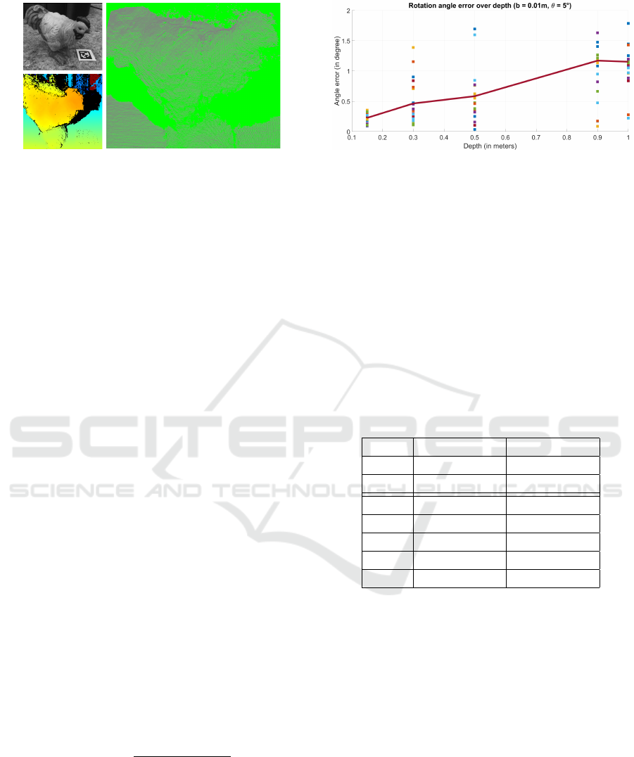
Figure 8: Dense 3D reconstruction of a small object by

monocular stereo vision.

5.3 Pose Estimation Evaluation

Accurate object pose estimation is crucial for all ma-

nipulation tasks, mainly when dealing with objects of

complex geometry. To investigate this, we analyzed

the impact of object rotations as a function of the cam-

era depth. Our objective is to demonstrate the neces-

sity of our distributed vision system for accurately es-

timating object poses, especially when handling small

objects. A ﬁxed movement baseline of 0.01 m was se-

lected for the robot, and the end-effector was rotated

by 5

◦

around a ﬁxed rotation axis to simulate object

rotation. This movement was performed at various

distances from the object, and only feature points on

the object were used. The angular error in the esti-

mated camera pose was analyzed, equivalent to a ro-

tation of the object when the camera is static.

Given a set of rotation matrices {R

}

i=1

with n be-

ing the number of runs for the same experiment, the

noise or error between these matrices can be quanti-

ﬁed by computing the angular deviation between each

matrix and a reference matrix, such as the mean ro-

tation matrix or a ground truth rotation matrix. If

no ground truth is available, the angular error can be

computed by ﬁrst estimating the mean rotation ma-

trix R

mean

from a set of rotation matrices {R

}

i=1

and afterward calculating the relative rotation error as

error,i

= R

⊤

mean

One way of calculating the mean rotation matrix

is by averaging the quaternions corresponding to each

rotation matrix.

The angular deviation between R

and R

mean

then calculated from the trace of R

error,i

= cos

−1



trace(R

error,i

) − 1



(12)

where θ

error,i

is the rotation angle (in rad) between

the matrices. The noise in the rotation matrices can

be quantiﬁed by computing the mean and standard

deviation of the angular errors θ

error,i

for all i. The

mean angular deviation θ

mean

provides a measure of

the average rotational error, while the standard devia-

Figure 9: Rotation angle error over depth to the investigated

object.

tion σ

quantiﬁes the noise in the set of rotation ma-

trices. The results are shown in Table 2 compared to

the angular error derived from the robot movement.

As expected, the robot shows an error independent

of the end-effector position (distance to the object),

while the estimation of the rotation via the camera

images deteriorates with increasing distance to the ob-

ject. This can also be observed in Figure 9, where the

error is shown as a function of depth. The points rep-

resent θ

error,i

whereas the red line represents θ

mean

different depths. This also reﬂects from Equation (6)

and Figure 4.

Table 2: Angle error of the estimated rotation angle between

two image captures.

Camera Robot

Depth θ

mean

± σ

mean

± σ

in m in

◦

0.15 0.227 ± 0.081 0.361 ± 0.021

0.30 0.464 ± 0.371 0.360 ± 0.019

0.50 0.585 ± 0.429 0.366 ± 0.040

0.90 1.172 ± 0.971 0.365 ± 0.039

1.00 1.154 ± 0.527 0.356 ± 0.005

From this, it can be concluded that having the ob-

ject as large as possible on the image scene is advan-

tageous for a precise object pose estimation. It is im-

possible to cover all parts of the workplace equally

with a static camera, making a system like ours indis-

pensable.

6 CONCLUSION

In this study, we proposed a ﬂexible distributed vi-

sion system for robot manipulation tasks. A static

depth camera gives a ﬁrst overview of the workspace.

By mounting an additional monocular camera on the

end-effector, it is possible to explore the entire robot

workspace. With this ﬂexible setup, it is possible to

adjust the decisive parameters for a 3D reconstruc-

Adaptable Distributed Vision System for Robot Manipulation Tasks

657

tion, such as the base width and the distance to the

analyzed scene, as desired. This theoretically en-

ables the entire working area of the robot to be re-

constructed with a high and, above all, consistent ac-

curacy. The system comprises two computing units

connected via Ethernet, allowing the 3D reconstruc-

tion process to be partitioned based on the speciﬁc re-

quirements of the intended application. To optimize

the system conﬁguration for the target application, a

self-evaluation framework was developed to assess re-

construction accuracy, speed, and latency for different

system conﬁgurations. For the hardware setup inves-

tigated during this work, the best results for sparse

3D reconstruction were achieved by running the fea-

ture detection on the embedded system and transmit-

ting the features to the central machine, where the re-

maining 3D reconstruction is performed. Both sparse

and dense reconstructions achieved errors in the mil-

limeter range. Future works aim to use the achieved

3D reconstruction for robotic manipulation tasks and

investigate reducing the processing and latency time

to use the system in a closed control loop. One pos-

sibility would be using a simple tracker that runs at

high speed on the embedded system in combination

with the robot’s state information and a Kalman Filter

to overcome the issue that the tracker only works for

small movements.

ACKNOWLEDGEMENTS

The authors acknowledge the ﬁnancial support by

the Bavarian State Ministry for Economic Affairs,

Regional Development and Energy (StMWi) for the

Lighthouse Initiative KI.FABRIK, (Phase 1: Infras-

tructure as well as research and development pro-

gram, grant no. DIK0249).

REFERENCES

Arruda, E., Wyatt, J., and Kopicki, M. (2016). Active

vision for dexterous grasping of novel objects. In

2016 IEEE/RSJ International Conference on Intelli-

gent Robots and Systems (IROS), pages 2881–2888.

Bay, H., Tuytelaars, T., and Van Gool, L. (2006). Surf:

Speeded up robust features. In Leonardis, A., Bischof,

H., and Pinz, A., editors, Computer Vision – ECCV

2006, pages 404–417. Springer Berlin Heidelberg.

Burschka, D. and Mair, E. (2008). Direct pose estimation

with a monocular camera. In Sommer, G. and Klette,

R., editors, Robot Vision, pages 440–453. Springer

Berlin Heidelberg.

Fern

andez Alcantarilla, P. (2013). Fast explicit diffusion for

accelerated features in nonlinear scale spaces.

Hagiwara, H. and Yamazaki, Y. (2019). Autonomous valve

operation by a manipulator using a monocular cam-

era and a single shot multibox detector. In 2019 IEEE

International Symposium on Safety, Security, and Res-

cue Robotics (SSRR), pages 56–61.

Hartley, R. and Zisserman, A. (2004). Multiple View Geom-

etry in Computer Vision. Cambridge University Press,

2 edition.

Hirschmuller, H. (2005). Accurate and efﬁcient stereo pro-

cessing by semi-global matching and mutual informa-

tion. In 2005 IEEE Computer Society Conference on

Computer Vision and Pattern Recognition (CVPR’05),

volume 2, pages 807–814 vol. 2.

Kappler, D., Meier, F., Issac, J., Mainprice, J., Ci-

fuentes, C. G., W

uthrich, M., Berenz, V., Schaal,

S., Ratliff, N. D., and Bohg, J. (2017). Real-time

perception meets reactive motion generation. CoRR,

abs/1703.03512.

Lin, Y., Tremblay, J., Tyree, S., Vela, P. A., and Birchﬁeld,

S. (2021). Multi-view fusion for multi-level robotic

scene understanding. In 2021 IEEE/RSJ International

Conference on Intelligent Robots and Systems (IROS),

pages 6817–6824.

Lowe, D. G. (2004). Distinctive image features from

scale-invariant keypoints. Int. J. Comput. Vision,

60(2):91–110.

McCormac, J., Clark, R., Bloesch, M., Davison, A. J., and

Leutenegger, S. (2018). Fusion++: Volumetric object-

level SLAM. CoRR, abs/1808.08378.

Murali, A., Mousavian, A., Eppner, C., Paxton, C., and Fox,

D. (2019). 6-dof grasping for target-driven object ma-

nipulation in clutter. CoRR, abs/1912.03628.

Nister, D. (2004). An efﬁcient solution to the ﬁve-point

relative pose problem. IEEE Transactions on Pattern

Analysis and Machine Intelligence, 26(6):756–770.

Redmon, J., Divvala, S. K., Girshick, R. B., and Farhadi, A.

(2015). You only look once: Uniﬁed, real-time object

detection. CoRR, abs/1506.02640.

Rosten, E. and Drummond, T. (2006). Machine learning

for high-speed corner detection. In Leonardis, A.,

Bischof, H., and Pinz, A., editors, Computer Vision

– ECCV 2006, pages 430–443. Springer Berlin Hei-

delberg.

Rublee, E., Rabaud, V., Konolige, K., and Bradski, G.

(2011). Orb: An efﬁcient alternative to sift or surf. In

2011 International Conference on Computer Vision,

pages 2564–2571.

Sch

onberger, J. L. and Frahm, J.-M. (2016). Structure-

from-motion revisited. In 2016 IEEE Conference on

Computer Vision and Pattern Recognition (CVPR),

pages 4104–4113.

Shahzad, A., Gao, X., Yasin, A., Javed, K., and Anwar,

S. M. (2020). A vision-based path planning and ob-

ject tracking framework for 6-dof robotic manipulator.

IEEE Access, 8:203158–203167.

Wang, T.-M. and Shih, Z.-C. (2021). Measurement and

analysis of depth resolution using active stereo cam-

eras. IEEE Sensors Journal, 21(7):9218–9230.

Zhang, Q., Cao, Y., and Wang, Q. (2023). Multi-vision

based 3d reconstruction system for robotic grinding.

In 2023 IEEE 18th Conference on Industrial Electron-

ics and Applications (ICIEA), pages 298–303.

VISAPP 2025 - 20th International Conference on Computer Vision Theory and Applications

658