Traffic Sign Orientation Estimation from Images Using Deep Learning
Raluca-Diana Chis¸
1 a
, Mihai-Adrian Loghin
1 b
, Cristina Mierl
˘
a
1 c
,
Horea-Bogdan Mures¸an
1 d
and Octav-Cristian Florescu
2
1
Department of Computer Science, Babes¸-Bolyai University, Cluj-Napoca, Romania
2
Grab, Geo Engineering, Vision, Cluj-Napoca, Romania
Keywords:
Yaw Estimation, Traffic Signs, Deep Learning.
Abstract:
This study presents our findings on estimating the horizontal rotation angle (yaw) of traffic signs from 2D
images using deep learning techniques. The aim is to introduce novel approaches for accurately estimating
a traffic sign’s orientation, with applications in automatic map generation. The primary goal is to associate
a traffic sign with a road correctly. The main challenge consists of both attempting to estimate the left/right
orientation of a sign from 2D images and accurately estimating the rotation of the sign in degrees. Our
approach involves the usage of a classifier for determining the orientation of a traffic sign in relation to the
observer. Furthermore, we tried to transfer the weights obtained from classification to regression models
and study the impact on performance. Our best results are obtaining an L1 loss as low as 10.34
◦
for yaw
estimation and an accuracy equal to 62% for orientation class assessment. The image data was obtained from
Grab’s Kartaview platform and was split into training/validation/testing while accounting for traffic sign class
and shape balancing.
1 INTRODUCTION
The main motivation behind our research is the need
to map traffic signs with their related roads cor-
rectly. According to Adewopo et al. (Adewopo et al.,
2023), T-intersections and four-way intersections are
the places with some of the highest traffic accident
rates and these are also the places with a high con-
glomeration of traffic signs, which can easily be mis-
interpreted. Our context is the following: Grab cre-
ates accurate maps, with the main focus on (but not
restricted to) the region of Southeast Asia, which are
then integrated into their application. One focus use
case of the applications is to offer GPS-navigation for
deliverers, thus driver’s safety and efficiency in traf-
fic are strongly related to the accuracy of the provided
maps. As such, GrabMaps is properly updated with
the latest changes in terms of traffic rules. Thousands
of images are collected from roads daily and any new
traffic signs are automatically detected.
In order to map a sign to a road, it is necessary
to know towards which road it is oriented (Figure 1).
a
https://orcid.org/0009-0000-0445-3961
b
https://orcid.org/0000-0001-6112-6713
c
https://orcid.org/0000-0002-2777-1353
d
https://orcid.org/0000-0003-4777-7821
The purpose of our research is to facilitate the soft-
ware that is able to compute the rotation angle (yaw)
of a traffic sign from a single 2-dimensional image.
This angle will be calculated as the yaw rotation rela-
tive to the heading of the camera that captured the im-
age. This research topic is particularly difficult since
in many cases even the human eye is unable to deter-
mine to which road a traffic sign is addressed.
Taking into consideration the state-of-the-art clas-
sification and regression models on angle and pose es-
timation, the following pre-trained models have been
applied: WideResNet (Zagoruyko and Komodakis,
2016), ResNext (Xie et al., 2016), Swin (Liu et al.,
2021). The results of the three models do not dif-
fer greatly, although certain particularities for each
model were observed. Experiments were conducted
with a set of 1617 images of traffic signs (provided
by Grab), manually annotated by us with orientation
classes (LEFT, RIGHT and CENTER) and with ro-
tation angles. One of our best results is a mean ab-
solute error equal to 10.34
◦
for yaw estimation with
the Swin Transformer model. Moreover, a 62% accu-
racy was obtained for the assessment of the orienta-
tion class with the ResNext model.
Regarding the structure of the paper, Section 2
presents the work of other researchers on yaw esti-
Chi¸s, R.-D., Loghin, M.-A., Mierl
ˇ
a, C., Mure¸san, H. B. and Florescu, O.-C.
Traffic Sign Orientation Estimation from Images Using Deep Learning.
DOI: 10.5220/0013115900003890
Paper published under CC license (CC BY-NC-ND 4.0)
In Proceedings of the 17th International Conference on Agents and Artificial Intelligence (ICAART 2025) - Volume 3, pages 233-240
ISBN: 978-989-758-737-5; ISSN: 2184-433X
Proceedings Copyright © 2025 by SCITEPRESS – Science and Technology Publications, Lda.
233

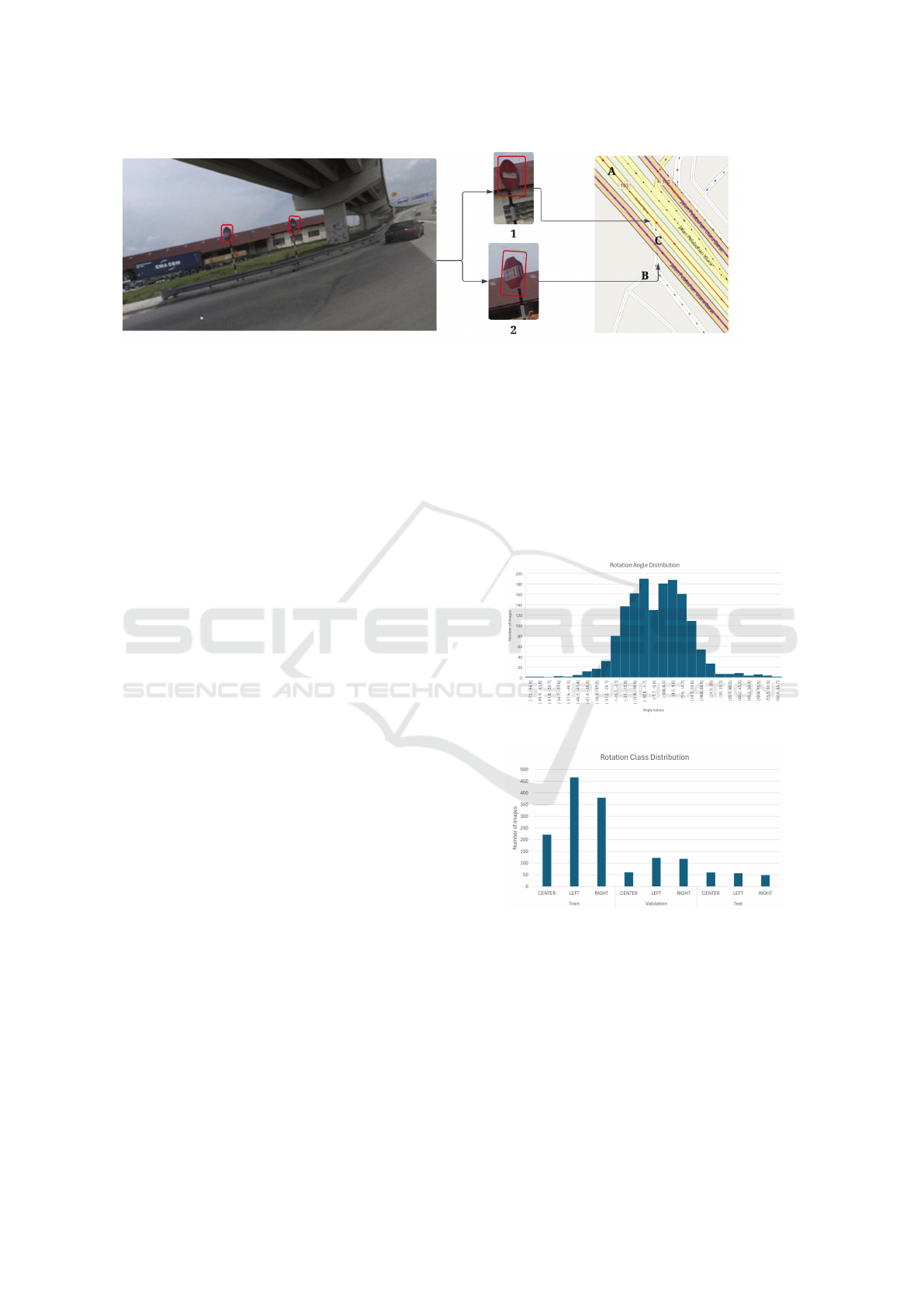
Figure 1: Visual explanation of the problem: users provide images from roads, traffic signs are identified, each sign is mapped
to a road according to its yaw rotation. In this case, sign 1 is mapped to road A, sign 2 to road B and C is the approximate
location of the picture.
mation. Section 3 describes the pre-processing tech-
niques applied to the dataset and our approach to the
proposed problem. Further, Section 4 presents the
performance of our experiments in comparison with
existing works. In the end, Section 5 summarizes our
findings and presents ideas for future improvements.
2 RELATED WORK
The detection of a sign and the identification of a
bounding box for it are crucial before orientation es-
timation. Approaches exist in 2D ((Hara et al., 2017),
(Raza et al., 2018)) or 3D ((Prisacariu et al., 2010),
(Kendall et al., 2015), (Mousavian et al., 2017)). Re-
search in orientation evaluation focuses on classifica-
tion and regression. Kanezaki et al. (Kanezaki et al.,
2018), Raza et al. (Raza et al., 2018), and Salas et
al. (Rodriguez Salas et al., 2021) propose the use of
convolutional neural networks for classification. In
(Kanezaki et al., 2018) an unsupervised model was
developed, called ”RotationNet”, that takes as input
multiple images with different perspectives on an ob-
ject and returns the object category and pose. In (Ro-
driguez Salas et al., 2021), the angle of rotation on the
Z-axis from a two-dimensional image is estimated,
using images from MNIST (Deng, 2012), rotated with
an angle between [0, 2π]. The angle values range
from -180
◦
to 180
◦
and were sampled in 16 classes.
(Raza et al., 2018) propose a CNN model to detect
pedestrian orientation using head pose and full-body
images. They achieved an accuracy of 0.91 for head
pose detection and 0.92 for full-body orientation.
In terms of using a regression-based approach,
Kendall et al. (Kendall et al., 2015) present a
CNN-based model, that uses transfer learning from
GoogLeNet (Szegedy et al., 2014) model. Another
relevant study that uses deep convolutional neural net-
works is described in (Hara et al., 2017), with the best
architecture based on the ResNet-101 model and pre-
trained weights. The results show a Mean Absolute
Error (MAE) value of 12.6
◦
for the EPFL Multi-view
Car Dataset (Ozuysal et al., 2009) and 30.2
◦
for the
TUD Multi-view Pedestrian Dataset (Andriluka et al.,
2010). Okorn et al. (Okorn et al., 2022) describe
a self-supervised method, which estimates the rela-
tive position of an object between neighboring objects
with Modified Rodrigues Projective Averaging.
Figure 2: Distribution of the yaw angle values.
Figure 3: Distribution of the rotation classes.
A particularly interesting approach to the prob-
lem is using several consecutive images of the same
sign. The SuperGlue (Sarlin et al., 2020) model pro-
poses an attentional graph neural network for match-
ing the key-points of two input images, thus enabling
cross-image communication. Similarly to PoseNet,
the study from (Cui et al., 2019) revolves around the
use of image pairs, whose features are extracted with
the SIFT and SURF algorithms, shifted and matched
correspondingly. An objective function is created for
ICAART 2025 - 17th International Conference on Agents and Artificial Intelligence
234

integrating these features in the 3D coordinate system,
which leads to the estimation of the traffic sign plane.
There are several approaches addressing the prob-
lem of orientation estimation. Although some re-
searchers employ multiple views of an object to esti-
mate its pose (Okorn et al., 2022), (Kanezaki et al.,
2018), a more practical and accessible method in-
volves using a single image of the object, as we pro-
pose in the following section. With a novel dataset
and stronger deep learning models, we provide an
original contribution to the state of the art of orien-
tation estimation.
3 METHODOLOGY
3.1 Dataset
The dataset used for provided by Grab, a major
player in the automatic mapping industry, contain-
ing images of traffic signs in Detroit, U.S.A. The
dataset includes 223619 images with varying de-
grees of quality, each containing at least a traffic
sign. There are 42 different traffic sign types, ranging
from TURN RESTRICTION U TURN LEFT US
to SPEED LIMIT 35 US. The dataset also contains
the bounding box of each sign in a rectangular shape,
revealing the approximate dimensions of the sign.
Due to the presence of multiple traffic signs and
significant background noise, the images underwent
cropping before initiating the training pipeline. The
best results were obtained using square images with
varying sizes, depending on the dimensions of the
traffic sign.
The process of manually annotating images ini-
tially included two rotation orientation classes (LEFT
and RIGHT) along with angle estimation. Upon fur-
ther review, an additional rotation class was intro-
duced to the dataset, categorizing front-facing images
into a new group called CENTER. This group en-
compasses images with rotation angles ranging be-
tween -5
◦
and 5
◦
, which are mostly imperceptible to
the human eye. This range was established empiri-
cally, based on observations from analyzing more im-
ages with low rotation angles and the results from ex-
plainability models for them.
The study aimed to compile a set of images ex-
hibiting a wide range of rotation angles, spanning
from front-facing orientations to extreme rotations.
Based on this criterion, a subset of the images was se-
lected. Still, a significant percentage (78.47%) of the
signs have a rotation angle between -30
◦
and 30
◦
(Fig.
2). However, the models struggle to categorize signs
with angles within this range due to small differences
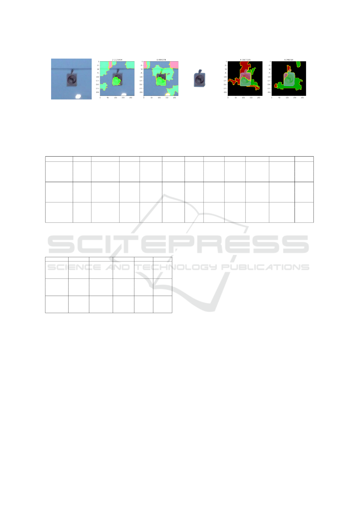
Figure 4: Example of background bias, caused by the mis-
match between the rotation of the power cable and of the
traffic sign.
in position. The quality of the images was also a cru-
cial criterion, as different individuals took pictures in
traffic while driving and using non-professional cam-
eras. Each image was manually verified to reduce
the likelihood of noisy inputs. The set contains 1534
records, with 26 traffic sign types and four categories:
square-shaped, wide rectangle, tall rectangle and sus-
pended rectangle. For experiments, the partitioning of
training, test, and validation sets was carried out con-
sidering the distribution of rotation orientation cate-
gories and sign types. Figure 3 displays the rotation
class distribution over the three image sets. 1069 im-
ages were selected for training, 301 for validation and
164 for testing.
Another relevant study direction was background
noise reduction. To achieve that, experiments were
performed with background-free images. To re-
move the background, the python library Back-
groundRemover
1
has been employed, which uses a
state-of-the-art model, hierarchical U-Net (Qin et al.,
2020). Removing backgrounds highlighted the im-
portance of image context and potential bias. An il-
lustrative example is shown in Figure 4. The left im-
age (a) shows a power cord suggesting central rota-
tion, while the sign itself appears rotated to the left. In
contrast, the image on the right (b) shows the traffic
sign isolated from the background, thus eliminating
potential confusion caused by the power cable.
3.2 Models
To tackle the challenge, models have been sought
out that are effective for both regression and clas-
sification tasks. These models were then subjected
to the procedure shown in Fig. 5. Considering the
approaches from the related literature, we have ob-
served the use of models based on ResNet-50 (Kogu-
ciuk et al., 2021) and also the use of convolutional
neural networks as the prime way to solve the prob-
lem (Kendall et al., 2015). We also aimed to study
1
https://pypi.org/project/backgroundremover/
Traffic Sign Orientation Estimation from Images Using Deep Learning
235

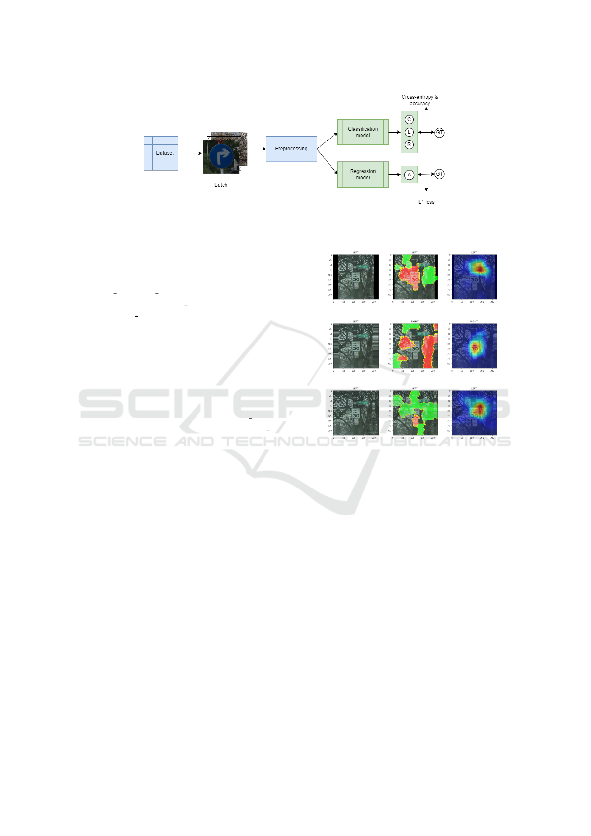
Figure 5: Diagram representing the process of sending the data through the classification (upper part) and regression models
(lower part), with the respective loss functions at the end. C, L and R stand for Center, Left and Right, respectively; A stands
for the angle predicted in terms of rotation degrees; GT stands for ground truth.
the impact of the model type and architecture on
the obtained results. Thus, we decided to use three
main models as the base of the research: WideRes-
Net (wide resnet101 2) (Zagoruyko and Komodakis,
2016), ResNext (resnext101 32x8d) (Xie et al., 2016)
and Swin (swin s) (Liu et al., 2021).
Swin Transformer was chosen as it is architec-
turally different from the other models that were used,
which contributed in the active learning process that
was used to obtain the regression data set. With this
diversity of the models in place, the process of ver-
ifying the quality of the labelled data became much
easier.
The models were implemented using PyTorch,
with initial weights from IMAGENET1K V2, for
WideResNet and ResNext, and IMAGENET1K V1,
for Swin. The weights were chosen based on the
best results from the available benchmarks for mod-
els. Our approach was based on transfer learning, the
most important part was to choose the most optimal
values for the base model and its options for training.
3.3 Quality Metrics
Given that we are approaching the problem from two
perspectives for pose estimation, classification and re-
gression, several metrics have been implemented to
evaluate our results. The metrics presented in this sec-
tion have been selected after multiple tests and con-
sidering the problem definition.
For the regression task we only considered the L1
loss function, known as mean absolute error (MAE)
(Hodson, 2022), to measure the results. This decision
was made since we needed an exact estimate as to
how far the model’s results were from the ground truth
in terms of degrees. As for the classification problem,
we utilised the categorical cross entropy (CCE) loss
function (Rusiecki, 2019; Wang et al., 2022), accu-
racy, precision, recall and f1-score to train and evalu-
ate the models.
(a) Original (b) LIME (c) GradCAM
(d) Original (e) LIME (f) GradCAM
(g) Original (h) LIME (i) GradCAM
Figure 6: LIME and GradCAM explanations given an im-
age with class left and several image augmentations. The
expectation is that a model will focus on the sign and its
edges. (a, b, c) show the results after constant padding, (d,
e, f) for edge padding, and (g, h, i) for reflection padding.
3.4 Explainability
To gain a better understanding of our results, we also
employed the use of two interpretation options for
the models. The decision was based on the fact that
large neural network models often present a black-
box decision-making process. As such, it is important
to understand why or if we should trust the decision-
making done by the models (Molnar, 2022; Selvaraju
et al., 2017; Ribeiro et al., 2016).
For both the regression and classification prob-
lems presented in the previous sections, we have gen-
erated explanations using LIME. This technique is
based on creating several interpretable models, such
as decision trees, and feeding them with variations of
the input data to gain an understanding of the impor-
tance of each feature (Molnar, 2022; Ribeiro et al.,
ICAART 2025 - 17th International Conference on Agents and Artificial Intelligence
236

2016). The explanations are presented in the form of
a mask with positive (green) and negative (red) impact
areas on the image for the given prediction (Molnar,
2022).
To gain an even better understanding, we also em-
ployed the use of another model-agnostic technique
known as GradCAM which was implemented specif-
ically for classification problems using neural net-
works. It brings several advantages since it offers
model-specific deterministic explanations. This tech-
nique is used by attaching the GradCAM explainer
to one of the layers of the model and only depend-
ing on the layer it is attached to will the explana-
tion change. The resulting explanation appears in the
form of a heatmap over the input image showcasing
the most important area for the given prediction (Sel-
varaju et al., 2017).
4 RESULTS
4.1 Classification Results
After analyzing the dataset, it was noticed that around
250 images could not be clearly characterized as left
or right. Those records were represented by signs
that were photographed front-facing the camera. In
order to organize the samples of the dataset into dis-
tinct classes we manually extracted and annotated the
images as a new class, CENTER. This addition was
relevant to the rotation class because it allows each of
the 3 classes to be more specialized in an angle rota-
tion interval. A rough estimation for the rotation class
CENTER interval is [-5, 5] degrees of rotation. This
improvement helped the model understand better that
a rotation angle closer to 0 leads to a front-facing sign,
while a rotation angle further away from 0 may indi-
cate one of the LEFT or RIGHT classes.
Several experiments have been conducted before
concluding that the best results would be for images
cropped directly in a square format, with and without
background (the notations ”bg” will be used for im-
ages with background, and ”no bg” for images with-
out background). After analyzing the models using
the previously mentioned explainers, it was noticed
that the models sometimes are misled by power lines
or other objects belonging to the background. With
this information, we believed that a model trained
on images without background has the capabilities to
better focus on the sign and its rotation, rather than
the background. The experiments were mainly run
for the classification part of the problem, which sim-
plifies the overall problem as previously stated. Some
of the results for different forms of image padding can
be observed in Fig. 6. The final experiments were
done on square images, specifically cropped this way
from the source image.
The Cross-entropy loss was used to evaluate the
models during training and the corresponding results
are displayed in Table 1. Optimizers Adam and
Stochastic Gradient Descent (SGD) have been used
alternatively with a learning rate (LR) equal to 3e-
5, which was set experimentally. The learning rate
scheduler from PyTroch StepLR has been applied
with a gamma factor equal to 0.1 and a step size of
7, implying that the LR has been decayed by a factor
of 0.1 every 7 epochs. All models have been trained
for 100 epochs, although the results are consistent af-
ter only 20 epochs. Regarding the sizes of the ex-
periment sets, they are constant (whether or not the
images have a background): the train set has 1069
images, the validation one 301 and the test set 164
images. The optimal found batch size was 4.
4.2 Regression Results
For the regression problem, we have only considered
experiments on images with and without background.
In our first experiments, we considered that the most
extreme scenarios could help us better understand the
model’s capabilities. The motivation for running ex-
periments on datasets with or without background is
similar to the one mentioned before, keeping the same
interpretations. As seen in Figure 7 the most accurate
results were obtained for a model trained on images
with background, but this was only the case for some
situations. Over multiple experiments, it has been no-
ticed that the no background model focuses better on
the sign. Another good aspect of the no background
model is that it does not give mainly negative numbers
for the results.
The optimizers, learning rate and scheduling use
the same hyperparameters as before. The loss func-
tion for the values presented in Table 2 is L1 (MAE)
loss. The models have been trained for 40 epochs,
as it was noticed that at this point the results stabi-
lize. The datasets used have the same size, with the
mention that the notations for the y-angle values were
used and the optimal batch size was 16.
4.3 Discussion
Before discussing the results, it is important to note
that the results in Tables 1 and 2 were the best over-
all results based on the best parameters found for
each model. The models were evaluated continu-
ously throughout the research as we corrected and
completed the dataset based on an active learning
Traffic Sign Orientation Estimation from Images Using Deep Learning
237

(a) Original (b) Background
model
(c) No background
model
(d) Original (e) Background
model
(f) No background
model
Figure 7: LIME results for an image considered in the centre class, with and without background, having a 3
◦
ground truth
rotation. The results in (b, e) are for a model only trained on images with background and the results in (c, f) are for a model
only trained on images without background.
Table 1: Experimental results for all three classification models under different optimizers and image inputs (bg - images with
full background; no bg - images that were processed and had their background removed, CE - Cross-entropy).
Model Optm. Image input Tr. Loss Val. Loss Test Loss Tr. Acc Val. Acc Test Acc Test Prec. Test Recall Test F1
WideResNet
SGD bg 1.01 1.00 1.05 0.51 0.52 0.48 0.48 0.48 0.48
SGD no bg 1.06 1.31 1.05 0.43 0.47 0.43 0.43 0.43 0.43
ADAM bg 2.59 1.43 1.66 0.46 0.45 0.43 0.43 0.43 0.43
ADAM no bg 0.89 1.04 1.34 0.58 0.52 0.40 0.38 0.38 0.38
ResNext
SGD bg 1.03 1.04 1.03 0.48 0.44 0.48 0.48 0.48 0.48
SGD no bg 1.02 49.72 1.03 0.48 0.48 0.48 0.48 0.48 0.48
ADAM bg 0.14 0.95 1.11 0.99 0.63 0.56 0.56 0.56 0.56
ADAM no bg 0.95 1.42 0.90 0.91 0.60 0.62 0.62 0.62 0.62
Swin
SGD bg 1.01 1.02 1.16 0.48 0.47 0.32 0.32 0.32 0.32
SGD no bg 1.01 1.02 1.13 0.46 0.45 0.35 0.35 0.35 0.35
ADAM bg 0.19 1.97 1.50 0.93 0.46 0.40 0.42 0.42 0.42
ADAM no bg 0.55 1.53 1.12 0.76 0.46 0.43 0.43 0.43 0.43
Table 2: Experimental results for all three regression mod-
els under different optimizers and image inputs (bg - images
with full background; no bg - images that their background
removed).
Model Optimizer Image input Train Loss Val. Loss Test Loss
WideResNet
SGD bg 13.59 12.91 10.35
SGD no bg 13.6 12.94 10.50
ADAM bg 6.93 11.85 11.00
ADAM no bg 9.49 11.65 10.59
ResNext
SGD bg 13.61 13.83 10.40
SGD no bg 13.60 13.55 10.39
ADAM bg 7.25 12.05 11.26
ADAM no bg 9.38 11.90 11.76
Swin
SGD bg 13.55 12.91 10.34
SGD no bg 13.50 12.80 10.37
ADAM bg 10.10 13.66 11.12
ADAM no bg 11.01 11.60 11.64
approach. Throughout this process, the model with
the best results changed continuously as more diverse
data was added. In the end, all the models obtained
similar results, indicating that the problem’s solution
is related directly to the quality of the data.
For the classification task, the most common best
performances were on the set of no-background im-
ages using the ADAM optimizer, with the best per-
formance being given by the model ResNext as in Ta-
ble 1. Most of the time the models ended up overfit-
ting easily on the training data set, obtaining results as
good as 0.99 at most, but the validation results stag-
gered at around 0.57 at most. The same drop in accu-
racy can also be seen in the test data for most of the
models. The drop in accuracy might be due to the dif-
ference in class balance between the subsets of data.
The type of the sign in the image did not affect the
performance of our models.
On the regression task, a similar situation can be
noticed by comparing the results in Table 2 and Fig.
7. This time WideResNet had the best performance
on training data and Swin for test data, but as before
the results were not that far apart between the models.
It might seem counter-intuitive that this time the re-
sults on the test data are better than that for the other
splits in some cases. This can be explained by the
distribution of the angle values in the dataset and how
they were further distributed between the subsets.
In addition to the numerical results, we also ob-
tained visual explanations via LIME and GradCAM.
In Fig. 6 we can see the explanations for the classi-
fication task using both approaches and in Fig. 7 the
explanations for the regression task only using LIME,
since GradCAM is classification-specific. Based on
the obtained explanations, we can conclude that the
models have successfully learned to identify objects
of interest for class and angle prediction, which back-
ground information confuses the model, and that
background removal is a useful tool for encouraging
this learned behavior.
Compared to other articles, the prediction of the
rotation class in terms of accuracy and loss might be
considered satisfactory. In (Rodriguez Salas et al.,
2021) the lowest error rate was equal to 0.93%, which
is higher than our smallest, 0.9%. Considering that
our best accuracy is 62% on test data, 63% on vali-
ICAART 2025 - 17th International Conference on Agents and Artificial Intelligence
238

dation data and 99% on training data, we could say
that it is worse than 91% from (Raza et al., 2018)
or 81.17% presented in (Kanezaki et al., 2018). We
consider two reasons for this: the difficulty of work-
ing with traffic signs for this task and the usage of
the CENTER class. Working with images depict-
ing objects with increased depth (such as humans in
(Raza et al., 2018) or cars, beds, mugs and so on in
(Kanezaki et al., 2018)), provides the benefit of hav-
ing more particular and easily categorizable sides of
an object. Traffic signs, on the other hand, tend to
be quite thin, and their left perspective does not differ
much visually from the right one.
The CENTER class represents a bridge between
the two other classes, and these images are harder
to classify due to their poorer representation in the
dataset. Of all images, only 22.35% belong to the
CENTER class. Moreover, in the train set 20.76% of
the images are centered and in the test set 36.58%,
which caused the CENTER category to have a greater
influence on the final results, although the models
were less trained for it. Our best model obtained on
the test set for the RIGHT category an accuracy of
73%, followed by the LEFT class with 61% and CEN-
TER with 34%. If we neglect the CENTER class, the
final accuracy would be 67%.
In terms of angle prediction, our degree of error
is much lower than that of multiple other research pa-
pers. As in the previous paragraph, the comparison
might not be as direct, given the usage of different
datasets, but it is still relevant to understanding the
true quality of the results. Given that the lowest error
in our case is equal to 10.34
◦
on the test, with a 6.93
◦
error on the train data, we are within the expected er-
ror rate, even below it. We are below the results of
articles such as (Cui et al., 2019), where the authors
obtained a mean error of 14.45
◦
, but above those of
article (Okorn et al., 2022). It is worth mentioning
that in (Okorn et al., 2022) the authors note a higher
error for images with more noise in them, something
that was addressed in this paper by using background
removal to eliminate the noise created by background
information. A smaller error rate was also obtained in
comparison with (Hara et al., 2017), where the MAE
value for the EPFL Multi-view Car Dataset (Ozuysal
et al., 2009) is 12.6
◦
and for the TUD Multi-view
Pedestrian Dataset (Andriluka et al., 2010) it is equal
to 30.2
◦
.
5 CONCLUSION AND FUTURE
WORK
Our work stands out from the others by using per-
forming deep/transfer learning methods and a manu-
ally annotated dataset. Our models have obtained an
MAE score as low as 10.34
◦
and an accuracy of up
to 62% on unseen data. Using the explainable mod-
els, LIME and GradCAM, provided a deeper under-
standing of the learning process and of the challenges
faced. Up to this point, conclusions have been derived
by separating the problem into regression and classi-
fication.
A main focus point in our research is the impact
of background information/noise on the angle and ro-
tation class prediction tasks. The experiments, at first
glance, have shown that removing the background in-
formation does not yield better or worse results, but
using explanation methods, we can determine that it
helps the models focus on the object of interest sig-
nificantly more. Based on the results from the images
with and without background, it can be seen that the
background noise does not affect the models’ perfor-
mance most of the time. The results, as evaluated in
comparison, tend not to have a strong deviation from
each other.
Some problems that were highlighted using the
LIME and GradCAM tools require further experimen-
tation and testing. Similarly, the impact of padding,
removing, or expanding the background for signs
must be explored in more depth, as it may lead to bet-
ter results for both classification and regression. Cur-
rently, we could only determine that it is much more
favorable to crop based on a square box around the
sign.
For further experiments, we plan on expanding the
problem solution with the use of a multitask model.
The model would supposedly have two heads: one
for classification and one for regression. Given the
results of the two heads, we plan to calculate the final
results as previously mentioned. Most of the problem
will come down to how the loss function is computed.
ACKNOWLEDGMENT
This research has been funded by Grab, as part of
a collaboration with Babes¸-Bolyai University. All
data used are the property of Grab, who provided
access for the authors to their data set through their
Kartaview platform of images captured with onboard
cameras on US roads.
Traffic Sign Orientation Estimation from Images Using Deep Learning
239

REFERENCES
Adewopo, V., Elsayed, N., ElSayed, Z., Ozer, M., Wangia-
Anderson, V., and Abdelgawad, A. (2023). Ai on the
road: A comprehensive analysis of traffic accidents
and autonomous accident detection system in smart
cities. In 2023 IEEE 35th International Conference on
Tools with Artificial Intelligence (ICTAI), pages 501–
506.
Andriluka, M., Roth, S., and Schiele, B. (2010). Monocular
3d pose estimation and tracking by detection. In 2010
IEEE Computer Society Conference on Computer Vi-
sion and Pattern Recognition, pages 623–630.
Cui, Z., Liu, Y., and Ren, F. (2019). Homography-based
traffic sign localization and pose estimation from im-
age sequence. IET Image Processing, 13.
Deng, L. (2012). The mnist database of handwritten digit
images for machine learning research. IEEE Signal
Processing Magazine, 29(6):141–142.
Hara, K., Vemulapalli, R., and Chellappa, R. (2017). De-
signing deep convolutional neural networks for con-
tinuous object orientation estimation.
Hodson, T. O. (2022). Root-mean-square error (rmse)
or mean absolute error (mae): when to use them or
not. Geoscientific Model Development, 15(14):5481–
5487.
Kanezaki, A., Matsushita, Y., and Nishida, Y. (2018). Ro-
tationnet: Joint object categorization and pose estima-
tion using multiviews from unsupervised viewpoints.
In Proceedings of the IEEE Conference on Computer
Vision and Pattern Recognition (CVPR).
Kendall, A., Grimes, M., and Cipolla, R. (2015). Posenet:
A convolutional network for real-time 6-dof camera
relocalization. CoRR, abs/1505.07427.
Koguciuk, D., Arani, E., and Zonooz, B. (2021). Perceptual
loss for robust unsupervised homography estimation.
In Proceedings of the IEEE/CVF Conference on Com-
puter Vision and Pattern Recognition (CVPR) Work-
shops, pages 4274–4283.
Liu, Z., Lin, Y., Cao, Y., Hu, H., Wei, Y., Zhang, Z., Lin,
S., and Guo, B. (2021). Swin transformer: Hierarchi-
cal vision transformer using shifted windows. CoRR,
abs/2103.14030.
Molnar, C. (2022). Interpretable Machine Learning. Lean-
pub, 2 edition.
Mousavian, A., Anguelov, D., Flynn, J., and Kosecka, J.
(2017). 3d bounding box estimation using deep learn-
ing and geometry.
Okorn, B., Pan, C., Hebert, M., and Held, D. (2022). Deep
projective rotation estimation through relative super-
vision.
Ozuysal, M., Lepetit, V., and Fua, P. (2009). Pose estima-
tion for category specific multiview object localiza-
tion. In 2009 IEEE Conference on Computer Vision
and Pattern Recognition, pages 778–785.
Prisacariu, V. A., Timofte, R., Zimmermann, K., Reid, I.,
and Van Gool, L. (2010). Integrating object detection
with 3d tracking towards a better driver assistance sys-
tem. In 2010 20th International Conference on Pat-
tern Recognition, pages 3344–3347.
Qin, X., Zhang, Z., Huang, C., Dehghan, M., Zaiane, O. R.,
and Jagersand, M. (2020). U2-net: Going deeper with
nested u-structure for salient object detection. Pattern
Recognition, 106:107404.
Raza, M., Rehman, S.-U., Wang, P., and Peng, B. (2018).
Appearance based pedestrians’ head pose and body
orientation estimation using deep learning. Neuro-
computing, 272:647–659.
Ribeiro, M. T., Singh, S., and Guestrin, C. (2016). ”why
should i trust you?”: Explaining the predictions of any
classifier. In Proceedings of the 22nd ACM SIGKDD
International Conference on Knowledge Discovery
and Data Mining, pages 1135–1144, New York, NY,
USA. Association for Computing Machinery.
Rodriguez Salas, R., Dokladal, P., and Dokladalova, E.
(2021). A minimal model for classification of rotated
objects with prediction of the angle of rotation. Jour-
nal of Visual Communication and Image Representa-
tion, 75:103054.
Rusiecki, A. (2019). Trimmed categorical cross-entropy for
deep learning with label noise. Electronics Letters, 55.
Sarlin, P.-E., DeTone, D., Malisiewicz, T., and Rabinovich,
A. (2020). Superglue: Learning feature matching with
graph neural networks.
Selvaraju, R. R., Cogswell, M., Das, A., Vedantam, R.,
Parikh, D., and Batra, D. (2017). Grad-cam: Visual
explanations from deep networks via gradient-based
localization. In 2017 IEEE International Conference
on Computer Vision (ICCV), pages 618–626.
Szegedy, C., Liu, W., Jia, Y., Sermanet, P., Reed, S.,
Anguelov, D., Erhan, D., Vanhoucke, V., and Rabi-
novich, A. (2014). Going deeper with convolutions.
Wang, Q., Ma, Y., Zhao, K., and Tian, Y. (2022). A compre-
hensive survey of loss functions in machine learning.
Annals of Data Science, 9(2):187–212.
Xie, S., Girshick, R. B., Doll
´
ar, P., Tu, Z., and He, K.
(2016). Aggregated residual transformations for deep
neural networks. CoRR, abs/1611.05431.
Zagoruyko, S. and Komodakis, N. (2016). Wide residual
networks. CoRR, abs/1605.07146.
ICAART 2025 - 17th International Conference on Agents and Artificial Intelligence
240