Topological Attention and Deep Learning Integration for Electricity

Consumption Forecasting

Ahmed Ben Salem

and Manar Amayri

2 a

Higher School of Communication of Tunis, Tunis, Tunisia

Concordia Institute for Information Systems Engineering (CIISE), Concordia University, Canada

Keywords:

Time Series Forecasting, Attention Mechanism, Persistent Homology, Deep Learning, Electricity

Consumption Forecasting.

Abstract:

In this paper, we consider the problem of point-forecasting of univariate time series with a focus on electricity

consumption forecasting. Most approaches, ranging from traditional statistical methods to recent learning-

based techniques with neural networks, directly operate on raw time series observations. The main focus of

this paper is to enhance forecasting accuracy by employing advanced deep learning models and integrating

topological attention mechanisms. Speciﬁcally, N-Beats and N-BeatsX models are utilized, incorporating var-

ious time and additional features to capture complex nonlinear relationships and highlight signiﬁcant aspects

of the data. The incorporation of topological attention mechanisms enables the models to uncover intricate and

persistent relationships within the data, such as complex feature interactions and data structure patterns, which

are often missed by conventional deep learning methods. This approach highlights the potential of combining

deep learning techniques with topological analysis for more accurate and insightful time series forecasting in

the energy sector.

1 RELATED WORK

Accurate electricity consumption forecasting is es-

sential for energy management, pricing, and distribu-

tion. Traditional methods, including statistical mod-

els such as ARIMA (Box et al., 2015) and exponential

smoothing (Winters, 1960), have been widely used

but often struggle with the nonlinear and complex

nature of time series data. Recent advances in deep

learning, such as Long Short-Term Memory (LSTM)

(Sherstinsky, 2020), Gated Recurrent Units (GRU)

(Sherstinsky, 2020), and N-Beats (Oreshkin et al.,

2019), have shown promise in capturing these nonlin-

ear relationships. However, most methods rely solely

on raw time series data and fail to leverage the under-

lying topological structure of the data.

This paper proposes the integration of topolog-

ical attention mechanisms into deep learning mod-

els to improve forecasting accuracy. By incorporat-

ing persistent homology and related techniques from

topological data analysis (TDA), the models can cap-

ture complex interactions within the data, provid-

ing a more holistic approach to time series forecast-

https://orcid.org/0000-0002-5610-8833

ing(Chazal and Michel, 2021).

Recent advancements in time series forecasting

have expanded beyond traditional statistical meth-

ods, integrating complex machine learning tech-

niques to handle the nonlinear and intricate nature of

data(Rebei et al., 2023; Rebei et al., 2024). In partic-

ular, integrating topological data analysis (TDA) into

forecasting models has garnered signiﬁcant attention

for its potential to enhance performance.

The N-Beats model, introduced by Oreshkin et

al. (Oreshkin et al., 2019), has shown considerable

promise by addressing some of the limitations of con-

ventional methods. This model’s ability to decom-

pose time series data into trend and seasonal compo-

nents through a fully connected network represents a

signiﬁcant step forward. Despite this progress, con-

ventional models, including N-Beats, often overlook

the underlying topological structures present in the

data.

To bridge this gap, Zhang et al. (Zeng et al., 2021)

pioneered the use of topological attention mecha-

nisms in forecasting models. Their work integrates

topological features, such as persistence diagrams, to

capture and leverage the persistent structures within

the data. This approach provides a more nuanced rep-

Ben Salem, A. and Amayri, M.

Topological Attention and Deep Learning Integration for Electricity Consumption Forecasting.

DOI: 10.5220/0013116800003953

Paper published under CC license (CC BY-NC-ND 4.0)

In Proceedings of the 14th International Conference on Smart Cities and Green ICT Systems (SMARTGREENS 2025), pages 15-23

ISBN: 978-989-758-751-1; ISSN: 2184-4968

resentation of the data’s complexity compared to tra-

ditional methods, which typically do not incorporate

such structural insights.

Further research by Chazal et al. (Chazal and

Michel, 2021) provides a comprehensive overview of

TDA techniques and their application to various do-

mains. Their work highlights the potential of persis-

tent homology in capturing the essential topological

features that inﬂuence time series behavior.

Although our approach is similar to that in (Li

et al., 2019) by utilizing self-attention, it diverges

in that the representations provided to the attention

mechanism are derived not from convolutions, but

from a topological analysis. This method inherently

captures the ”shape” of local time series segments

through its construction.

In summary, integrating TDA with deep learning

models represents a promising approach to overcom-

ing the limitations of traditional forecasting methods.

By leveraging topological features, these enhanced

models can provide deeper insights into data struc-

ture and improve predictive accuracy across a range

of applications.

2 METHODOLOGY

2.1 N-Beats and N-BeatsX Models

2.1.1 Overview of NBeats Model

The NBeats model, introduced by Oreshkin et al.

(2019) (Oreshkin et al., 2019), is a deep learning ar-

chitecture designed for time series forecasting. It op-

erates using a stack of fully connected layers orga-

nized into blocks. Each block performs two key op-

erations: backcasting (reconstructing the input) and

forecasting (predicting future values).

2.1.2 Input and Output of Each Block

For block i, the input is the residual from the previ-

ous block. Let x

(i)

denote the input to block i. The

block generates two outputs: the backcast b

(i)

and the

forecast f

(i)

= g



(i)

;θ

(i)



, (1)

(i)

= g



(i)

;θ

(i)



, (2)

where g

(·) and g

(·) are fully connected networks

with parameters θ

(i)

and θ

(i)

, respectively. The input

to the next block is the residual, calculated as:

(i+1)

= x

(i)

−b

(i)

. (3)

2.1.3 Input and Output of the Stack

Each stack in the NBeats model consists of multiple

blocks that work together to reﬁne the residuals and

produce forecasts. The input to each stack s is the

residual from the previous stack, denoted as x

(s)

. In-

side the stack, the blocks process the input sequen-

tially, generating both backcasts and forecasts. The

forecast output of each stack is the sum of the fore-

casts from all blocks within the stack:

(s)

∑

i=1

(s,i)

, (4)

where f

(s,i)

represents the forecast produced by block

i in stack s and K

is the number of blocks in the stack

s. The input to the next stack is the residual after back-

casting, calculated as:

(s+1)

= x

(s)

−

∑

i=1

(s,i)

. (5)

Thus, each stack progressively reﬁnes the residuals

from the previous stack and contributes to the overall

forecast.

2.1.4 Input and Output of the Entire Model

As illustrated in Figure 1, the NBeats model is com-

posed of multiple stacks, each responsible for captur-

ing different components of the time series, such as

trend and seasonality in the case of the interpretable

model. The ﬁnal forecast of the entire model is ob-

tained by summing the forecasts from all stacks:

y =

∑

s=1

(s)

∑

s=1

∑

i=1

(s,i)

, (6)

where M is the total number of stacks and

(s)

is the

forecast generated by stack s. This multi-stack archi-

tecture allows the model to learn hierarchical repre-

sentations of the time series, with each stack captur-

ing different temporal patterns or features.

In the interpretable model, the stacks are special-

ized to capture speciﬁc components such as trend and

seasonality. In contrast, the generic model allows the

stacks to learn more ﬂexible and general representa-

tions of the time series data.

2.2 Overview of NBeatsX Model

In the following section, we explore the NBeatsX

model, an extension of the original NBeats model that

incorporates exogenous variables X. We discuss how

NBeatsX builds upon the NBeats architecture to han-

dle external inﬂuences and the implications of these

modiﬁcations for time series forecasting.

SMARTGREENS 2025 - 14th International Conference on Smart Cities and Green ICT Systems

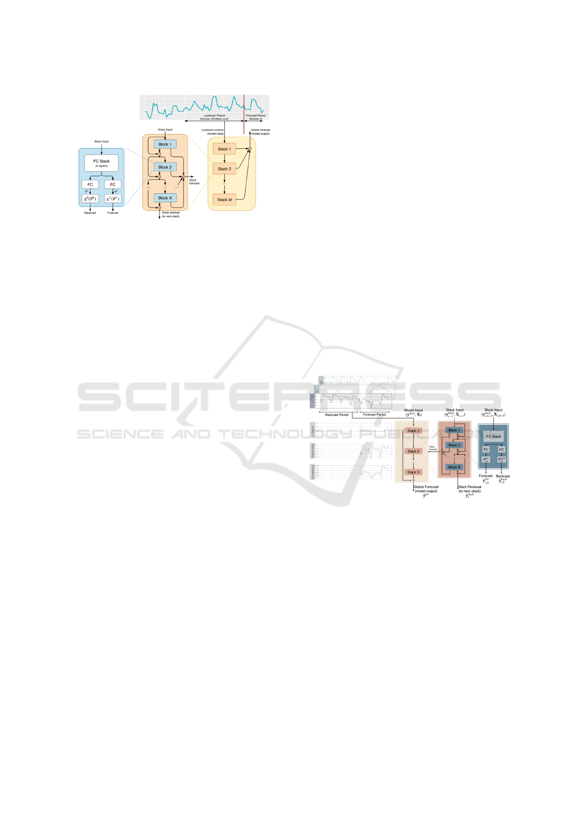
Figure 1: Architecture of the NBeats model (Oreshkin et al.,

2019).

2.2.1 Input and Output of Each Block

The input and output structure of each block in

NBeatsX is similar to that of NBeats, with the key

difference being the inclusion of exogenous variables

(i)

in the input. For block i, the input now includes

both the residual from the previous block and the ex-

ogenous variables. The block generates two outputs:

the backcast b

(i)

and the forecast f

(i)

= g



(i)

, X

(i)

;θ

(i)



, (7)

(i)

= h



(i)

, X

(i)

;θ

(i)



, (8)

where g(·) and h(·) are fully connected networks with

parameters θ

(i)

and θ

(i)

, respectively. The input to the

next block is the residual, calculated as:

(i+1)

= x

(i)

−b

(i)

. (9)

2.2.2 Input and Output of Each Stack

The stacking structure in NBeatsX follows the same

principles as in NBeats, with each stack consisting

of multiple blocks that process the input sequentially.

The key difference lies in how the exogenous vari-

ables X

(s)

are integrated into each stack. In NBeatsX,

each stack takes both the residuals and the exogenous

variables as inputs:

(s)

∑

i=1

(s,i)

, (10)

where f

(s,i)

represents the forecast produced by block i

in stack s, and the exogenous variables X

(s)

contribute

to the forecasting process. The input to the next stack

is the residual after backcasting, calculated as:

(s+1)

= x

(s)

−

∑

i=1

(s,i)

. (11)

2.2.3 Input and Output of the Entire Model

As illustrated in Figure 2, the NBeatsX model is com-

posed of multiple stacks, each responsible for captur-

ing different components of the time series, while also

considering the inﬂuence of exogenous variables. The

ﬁnal forecast of the entire model is obtained by sum-

ming the forecasts from all stacks:

y =

∑

s=1

(s)

∑

s=1

∑

i=1

(s,i)

, (12)

where M is the total number of stacks, K

is the num-

ber of blocks in stack s, and

(s)

is the forecast gener-

ated by stack s. The inclusion of exogenous variables

allows the NBeatsX model to capture additional tem-

poral patterns and external inﬂuences, enhancing its

forecasting accuracy.

In the interpretable version of NBeatsX, the stacks

can be specialized to capture speciﬁc components of

the time series, such as trend and seasonality, while

also accounting for the effects of exogenous variables.

The generic model version allows for more ﬂexible

representations of the time series data, adapting to

various external factors.

Figure 2: Architecture of the NBeatsX model (Olivares

et al., 2023).

3 TOPOLOGICAL ATTENTION

In this section, we explore the integration of topolog-

ical attention into deep learning models, focusing on

persistent homology and its vectorization for use in

Transformer architectures.

3.1 Persistent Homology and Barcode

Calculation

Persistent homology is computed from time series

data segmented into overlapping windows. Each win-

dow is converted into a point cloud using time-delay

Topological Attention and Deep Learning Integration for Electricity Consumption Forecasting

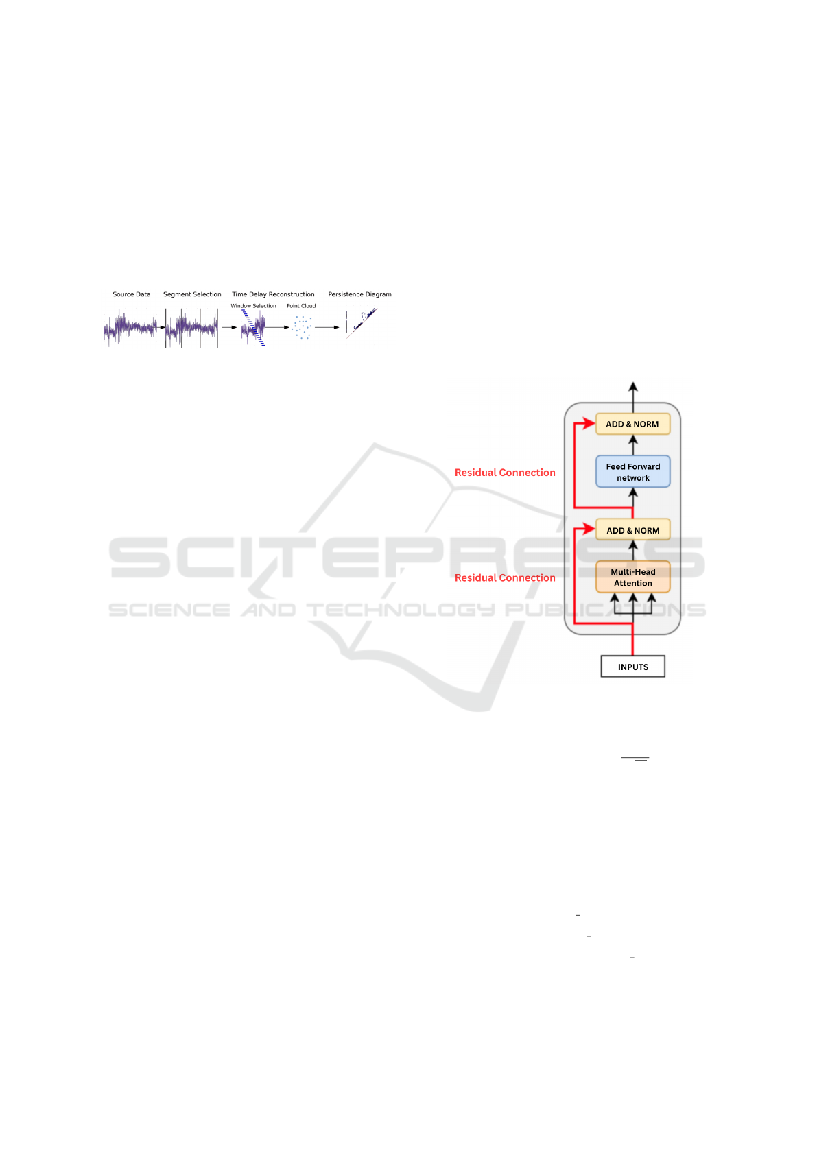
embedding (Seversky et al., 2016). The point cloud is

deﬁned as:



, x

t+τ

, x

t+2τ

, . . . , x

t+(d−1)τ



(13)

where τ is the delay and d is the embedding di-

mension. Persistent homology is computed using

the Ripser algorithm (Bauer, 2021), yielding bar-

codes that summarize topological features such as

connected components and loops.

Figure 3: Process of calculating persistent homology for

time series data.

3.2 Barcode Vectorization

Many approaches have been proposed to alleviate this

issue, including ﬁxed mappings into a vector space

(Adams et al., 2017), Kernel techniques (Reininghaus

et al., 2015), and learnable vectorization schemes, the

latter of which we have employed as it integrates well

into the regime of neural networks (Carri

ere et al.,

2020).

Persistence barcodes are mapped into a vector

space using differentiable functions. The vectoriza-

tion involves several steps:

1. Barcode Coordinate Function: Transform each

pair (b

, d

) using functions such as Gaussian ker-

nel:

, d

) = exp



−

−b

)

2θ



(14)

and Linear weighting:

, d

) = θ(d

−b

) (15)

2. Summing over Barcode: Aggregate the trans-

formed values:

(B) =

∑

i=1

, d

) (16)

3. Multiple Parameters: Compute vectorization for

multiple θ values:

V(B) = (V

(B), V

(B), . . . , V

(B)) (17)

where θ ∈ {0.1, 0.2, 0.25, 0.3, 0.5, 0.6, 0.75, 0.85,

0.9, 1.0}, representing the 10 distinct values of θ

used in this study.

4. Combining Multiple Functions: Concatenate

results from different functions:

ﬁnal

(B) =



(B), V

(B), . . . , V

(B)



(18)

Thus, the persistence barcode is transformed into

a high-dimensional vector by applying different pa-

rameterized mappings, each of which emphasizes dis-

tinct features of the topological data.

3.3 Integration with Attention

Mechanism

The vectorized barcodes are integrated into a

Transformer-based architecture, speciﬁcally using the

encoder part of the Transformer model (Vaswani,

2017). The Transformer Encoder Layer processes the

input through multi-head self-attention and a feed-

forward network to capture the complex patterns in

the data.

Figure 4: Transformer Encoder Layer.

The multi-head attention mechanism is deﬁned as:

Attention(Q, K, V ) = softmax



⊤

√



V (19)

and extends to:

MultiHead(Q, K, V ) = Concat(head

, . . . , head

(20)

Transformer Encoder Parameters

Key parameters include:

• Number of layers (num layers = 4)

• Model dimensionality (d model = 128)

• Number of attention heads (num heads = 8)

• Feed-forward network size (dff = 256)

SMARTGREENS 2025 - 14th International Conference on Smart Cities and Green ICT Systems

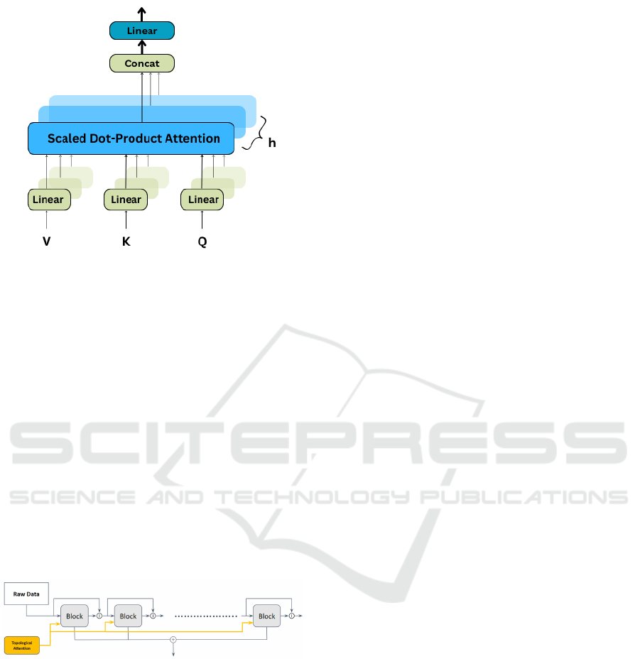
Figure 5: Multi-head Attention Mechanism.

3.4 Integrating Topological Attention

into Forecasting Models

The integration of topological attention into models

like NBeats enhances their ability to capture complex

temporal patterns by leveraging topological features.

As shown in Figure 6, we enrich the input signal to

each block by concatenating the topological attention

vector:

(i)

aug

(i)

, ν

(i)

where x

(i)

aug

is the augmented input to block i, and

(i)

is the topological attention vector. The topologi-

cal features, illustrated by the yellow arrows, provide

additional structural information, improving forecast-

ing accuracy.

Figure 6: Integration of topological attention into the

NBeats model.

4 DATA

4.1 INP Grenoble Dataset

4.1.1 Data Description

The INP Grenoble dataset is a private dataset from

a lab at the Grenoble Institute of Technology (INP

Grenoble) (A.P.I., ; Martin Nascimento et al., 2023).

It contains electricity consumption data recorded

from January 1, 2016, to May 10, 2022, with sam-

ples taken at one-hour intervals. This dataset provides

valuable insights into electricity usage patterns, which

can be useful for various energy-related applications.

4.1.2 Data Preprocessing

The INP Grenoble dataset, sourced from a single

building, contains inherent noise due to various un-

controllable factors like sensor accuracy and external

inﬂuences on electricity consumption. This higher

level of noise makes the dataset more challenging to

work with compared to others. Signiﬁcant prepro-

cessing steps were taken to handle missing data, out-

liers, and inconsistencies.

4.2 AEMO Australian Dataset

4.2.1 Data Description

The Australian Energy Market Operator (AEMO)

oversees Australia’s electricity and gas markets. It

provides public datasets containing electricity con-

sumption and price data for different regions across

Australia. One key dataset includes electricity de-

mand, recorded at 30-minute intervals, starting from

1998 (Australian Energy Market Operator, 2024).

This dataset is rich in historical data and offers a

broad view of national consumption trends (Operator,

2024).

4.2.2 Data Preprocessing

The AEMO dataset provides electricity consump-

tion data known as TOTAL DEMAND, measured in

megawatts (MW). Compared to the INP Grenoble

dataset, this dataset is much cleaner, as it spans a

larger population and features fewer inconsistencies.

Minimal preprocessing was required, primarily fo-

cused on handling missing values.

4.3 Exogenous Variables

The following exogenous variables were incorporated

into the N-BeatsX model to enhance its predictive

performance by leveraging external factors inﬂuenc-

ing electricity consumption.

4.3.1 Weather Features

For both datasets, weather-related features were col-

lected using the Open-Meteo API (Open-Meteo,

2024), with data covering the period from January 1,

2016, to December 31, 2019. To retrieve the weather

Topological Attention and Deep Learning Integration for Electricity Consumption Forecasting

data, the geographical location was passed as input to

the API.

For the INP Grenoble Dataset, the exact loca-

tion of the building was used to obtain precise weather

data, while for the AEMO Victoria Dataset, only the

general location of the city was considered.

Using the geographical coordinates of the respec-

tive regions, hourly weather data was obtained, in-

cluding variables such as temperature, humidity, pre-

cipitation, snow depth, cloud cover, and wind speed.

To improve predictive performance, an initial set

of features was reﬁned through a correlation study us-

ing correlation matrices. This allowed us to identify

and remove features with weak correlations to elec-

tricity consumption or high intercorrelation with other

variables.

• INP Grenoble Dataset: The ﬁnal set of selected

weather features includes temperature at 2 meters,

relative humidity at 2 meters, precipitation, and

wind speed at 10 meters.

• AEMO Victoria Dataset: The reﬁned weather

features include temperature at 2 meters, precipi-

tation, and wind speed at 10 meters.

This feature selection process aimed to ensure that

only the most relevant and non-redundant predictors

were used in the model, despite their relatively low

direct correlations with electricity consumption.

4.3.2 Time Features

In addition to weather data, temporal attributes were

derived from time columns to capture seasonality and

time-dependent patterns. These features include:

• Day of the Week: Indicates the day (e.g., Monday

to Sunday).

• Month and Season: Captures monthly and sea-

sonal variations.

• Day of the Year: Represents the position of the

day within the year.

• Weekend and Working Day Flags: Differentiates

between weekends and weekdays.

• Holiday Flags: Highlights speciﬁc holidays based

on predeﬁned lists for France and Australia.

These features were instrumental in enabling the

model to account for periodic trends and variations

speciﬁc to each dataset.

Comparison: While both datasets offer valuable

insights into electricity consumption, the INP Greno-

ble dataset exhibits signiﬁcantly more noise due to the

granularity and the single-building source, making it

more challenging to analyze compared to the AEMO

dataset, which is more stable and consistent.

5 RESULTS AND EVALUATION

5.1 Evaluation Metrics

We assess model performance using Root Mean

Squared Error (RMSE), Mean Absolute Error

(MAE), Symmetric Mean Absolute Percentage Error

(SMAPE), Correlation, and R-squared (R²). These

metrics offer a comprehensive evaluation of accuracy

and model ﬁt. RMSE and MAE focus on error mag-

nitudes, while SMAPE provides percentage-based er-

ror. Correlation measures the linear relationship be-

tween predictions and actual values, and R² assesses

the proportion of variance explained by the model.

5.2 Training and Hyperparameter

Tuning

Hyperparameter tuning plays a crucial role in opti-

mizing the performance of deep learning models. For

this paper, we employed the Hyperband tuning algo-

rithm (Li et al., 2018) to ﬁnd the best set of hyper-

parameters for the interpretable NBeats and NBeatsX

models.

In our training process, we focused on predict-

ing electricity consumption 24 hours ahead, aiming

to provide accurate forecasts for this short-term hori-

zon. Additionally, we conducted a search for the op-

timal lookback window and determined that a 7-day

lookback window is the ideal choice. This window

effectively captures the temporal patterns and season-

ality in the data, enhancing the models’ forecasting

performance.

5.3 Models Performance on AEMO

Dataset

Table 1 illustrates the performance of six different

models evaluated on the AEMO Australian dataset.

Table 1: Performance Metrics for Different Models on

AEMO Australian Dataset for 24-hour Forecasting.

Model MAE RMSE SMAPE Correlation R

GRU 519.06 703.97 10.86 0.46 0.14

LSTM 648.23 861.77 13.64 0.31 0.11

1D-CNN 303.24 466.54 6.27 0.78 0.62

LSTM-Attention 626.58 784.82 13.12 0.05 0.06

NBEATS+TopoAttn 328.85 428.32 6.81 0.82 0.67

NBEATSX+TopoAttn 161.72 217.88 2.96 0.93 0.89

The NBEATSX+TopoAttn model exhibits the

best overall performance, achieving the lowest MAE

of 161.72, the lowest RMSE of 217.88, and the lowest

SMAPE of 2.96%. This model also shows the highest

correlation of 0.93 and the highest R

score of 0.89,

indicating a strong ﬁt to the data and high acc uracy

SMARTGREENS 2025 - 14th International Conference on Smart Cities and Green ICT Systems

in predictions. Notably, NBEATSX+TopoAttn out-

performs the NBEATS+TopoAttn model, highlight-

ing the beneﬁt of incorporating exogenous variables

into the model. In comparison, the 1D-CNN model

also performs well but does not achieve the same level

of accuracy as the NBEATSX+TopoAttn model. The

LSTM and LSTM-Attention models show higher er-

rors and lower R

scores, reﬂecting their compara-

tively weaker performance.

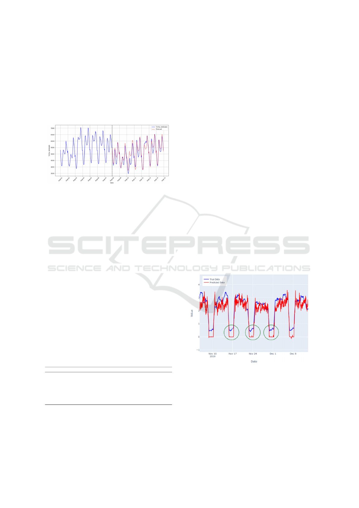
Figure 7: Actual vs. Forecasted Electricity Demand on

AEMO Dataset.

Figure 7 illustrates the actual total demand (blue

line) and the forecasted values (red dashed line) for

the AEMO Australian dataset over a period in August.

The black dashed vertical line represents the point

where the model starts generating forecasts. The close

alignment between the forecasted and actual values,

demonstrates the effectiveness of the model in cap-

turing the trends and variations in electricity demand.

Notably, the model performs well in predicting both

the peaks and troughs

5.4 Models Performance on INPG

Dataset

The same evaluation metrics used for the AEMO

Australian dataset are applied on the INP Grenoble

Dataset to compare the models’ accuracy and effec-

tiveness on this more challenging dataset. Table 2

shows how the different models performed on the INP

Grenoble dataset.

Table 2: Performance Metrics for Different Models on INP

Grenoble Dataset for 24-hour Forecasting.

Model MAE RMSE SMAPE Correlation R

GRU 0.79 1.14 127.29 0.793 0.56

LSTM 1.013 1.35 92.68 0.632 0.37

1D-CNN 0.81 1.17 122.30 0.776 0.54

LSTM-Attention 0.83 1.20 124.07 0.766 0.52

HyDCNN 0.88 1.26 123.93 0.752 0.62

NBEATS+TopoAttn 0.42 0.77 23.98 0.784 0.70

NBEATSX+TopoAttn 0.79 1.12 83.98 0.781 0.57

The GRU model shows the best correlation of

0.793 on the INP Grenoble dataset, indicating it cap-

tures the relationships in the data most effectively.

However, the NBEATS+TopoAttn model achieves

the lowest MAE of 0.42, the smallest RMSE of 0.77,

and the lowest SMAPE of 23.98%. This model also

exhibits a high correlation of 0.784 and the best R

score of 0.70, indicating a very good ﬁt and high ac-

curacy in its predictions.

In comparison, the NBEATSX+TopoAttn model

also performs well, but has a higher MAE of 0.79,

RMSE of 1.12, and SMAPE of 83.98%. Its correla-

tion of 0.781 and R

of 0.57 are slightly lower, sug-

gesting that while this model is effective, it does not

perform as well as the NBEATS+TopoAttn model.

Other models such as GRU, 1D-CNN, LSTM,

LSTM-Attention, and HyDCNN show higher error

metrics and lower R

scores, indicating their relative

inferiority in performance.

Overall, the NBEATS+TopoAttn model stands

out as the most effective for this dataset, providing

the most accurate forecasts and illustrating the bene-

ﬁts of combining NBEATS with topological attention

techniques.

Performance Comparison: NBEATS

+TopoAttn vs. NBEATSX + TopoAttn

This section provides an in-depth analysis of why

the NBEATS+TopoAttn model outperforms the

NBEATSX+TopoAttn model on the INP Grenoble

dataset, despite the latter’s ability to capture speciﬁc

periods such as weekends and holidays.

Figure 8: NBEATS+TopoAttn model predictions on INP

Grenoble dataset. The green circles highlight the periods

where the model fails to capture weekends and holidays.

The NBEATS+TopoAttn model demonstrates su-

perior performance on the INP Grenoble dataset, with

the best metrics across all key indicators, as shown in

Table 2. However, a deeper examination of the pre-

dictions reveals some critical insights.

As shown in Figure 8, the NBEATS+TopoAttn

model tends to miss predictions during weekends and

Topological Attention and Deep Learning Integration for Electricity Consumption Forecasting

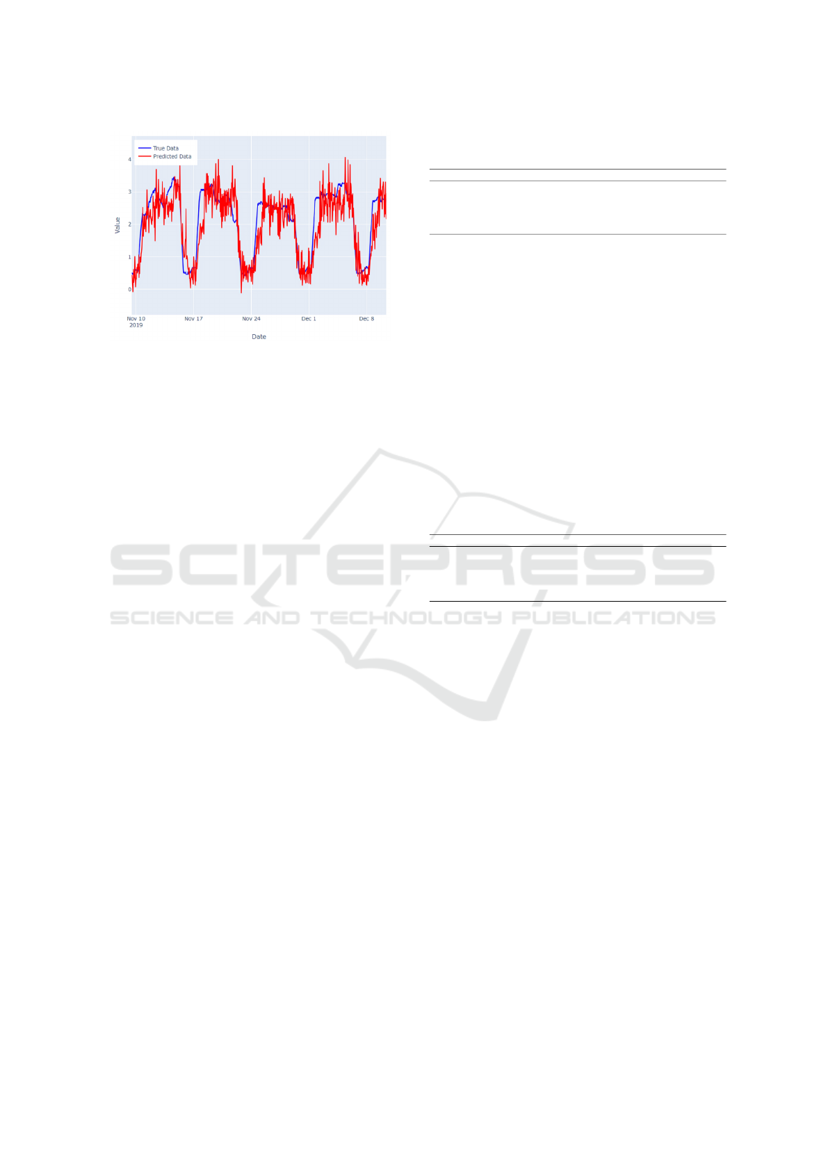
Figure 9: NBEATSX+TopoAttn model predictions on INP

Grenoble dataset.

holidays (highlighted with green circles), which con-

tributes to lower accuracy in these speciﬁc periods.

On the other hand, Figure 9 demonstrates that the

NBEATSX+TopoAttn model, which integrates time

and weather features, better captures these periods.

However, this comes at the cost of introducing more

noise throughout the entire dataset, which increases

the overall error metrics.

This trade-off explains why the NBEATS +

TopoAttn model outperforms the NBEATSX +

TopoAttn model in terms of MAE, RMSE, and

SMAPE, even though the latter model shows slightly

better performance in capturing the weekend and hol-

iday effects. The increased noise in the NBEATSX +

TopoAttn model diminishes its effectiveness in other

areas, resulting in a lower R

score and higher overall

error metrics.

6 ABLATION STUDY

An ablation study is a method used to evaluate the im-

portance of individual components within a complex

system. It involves systematically removing or deac-

tivating these components and observing the resulting

impact on the system’s overall performance.

In this section, we conduct an ablation study

on both the AEMO Australian dataset and the INP

Grenoble dataset. The study involves isolating and

analyzing the effect of topological attention and other

key features integrated into the NBeats and NBeatsX

models.

6.1 Ablation Study on AEMO Dataset

The ablation study on the AEMO dataset (see Table 3)

reveals key insights into the N-Beats and N-BeatsX

models. The baseline N-Beats model, without at-

Table 3: Ablation Study Results on AEMO Australian

Dataset.

Model Correlation R

RMSE MAE SMAPE

N-Beats 0.78 0.60 492.31 338.16 6.98

N-Beats+Attn 0.82 0.67 417.99 321.90 6.60

N-Beats + topoAttn 0.82 0.67 428.32 328.85 6.81

N-BeatsX 0.91 0.90 257.85 181.47 3.64

N-BeatsX + topoAttn 0.93 0.89 217.88 161.72 2.96

tention mechanisms or topological features, shows

poor performance (correlation: 0.78, RMSE: 492.31,

MAE: 338.16). Adding standard attention (N-Beats

+ Attn) improves results signiﬁcantly (correlation:

0.82, RMSE: 417.99, MAE: 321.90). Topological at-

tention (N-Beats + topoAttn) provides only marginal

gains. The N-BeatsX model, which includes exoge-

nous variables, performs better (correlation: 0.91,

RMSE: 257.85, MAE: 181.47). The best results come

from N-BeatsX + topoAttn, which achieves the low-

est errors and highlights the beneﬁts of combining ex-

ogenous variables with topological attention.

6.2 Ablation Study on INP Grenoble

Dataset

Table 4: Ablation Study Results on INP Grenoble Dataset.

Model Correlation R

RMSE MAE SMAPE

N-Beats 0.656 0.41 1.31 0.94 103.76

N-Beats+Attn 0.713 0.69 0.79 0.43 127.64

N-Beats + topoAttn 0.784 0.70 0.77 0.42 23.98

N-BeatsX 0.356 0.11 1.69 1.20 118.24

N-BeatsX + topoAttn 0.781 0.57 1.12 0.79 83.98

The ablation study on the INP Grenoble dataset

(see Table 4) reveals key ﬁndings about model com-

ponents. The baseline N-Beats model, without at-

tention or topological features, has moderate perfor-

mance (correlation: 0.656, RMSE: 1.31) but a high

SMAPE of 103.76%.

Adding standard attention (N-Beats + Attn) im-

proves RMSE to 0.79 and MAE to 0.43, with a cor-

relation of 0.713, though SMAPE rises to 127.64%,

indicating some instability.

Topological attention (N-Beats + topoAttn)

achieves the best results among N-Beats variants (cor-

relation: 0.784, RMSE: 0.77, MAE: 0.42, SMAPE:

23.98%), demonstrating effective use of topological

features.

The N-BeatsX model, with exogenous variables

but no attention, performs poorly (correlation: 0.356,

RMSE: 1.698, MAE: 1.20, SMAPE: 118.24%).

Adding topological attention (N-BeatsX + topoAttn)

improves correlation to 0.781, but RMSE (1.12) and

MAE (0.79) remain below the N-Beats + topoAttn

model, with SMAPE at 83.98%.

Overall, N-Beats + topoAttn outperforms N-

BeatsX + topoAttn, highlighting the N-Beats

SMARTGREENS 2025 - 14th International Conference on Smart Cities and Green ICT Systems

model’s superior ability to leverage topological fea-

tures for better performance on the INP Grenoble

dataset.

7 CONCLUSION

This paper focused on enhancing electricity consump-

tion forecasts using deep learning models with topo-

logical attention. We used N-Beats and N-BeatsX

models with topological attention on the AEMO Aus-

tralian and INP Grenoble datasets to test their robust-

ness.

On the AEMO dataset, N-BeatsX with exoge-

nous variables and topological attention outperformed

baseline models in MAE, RMSE, and SMAPE by

capturing complex patterns and external factors like

weather. For the noisier INP Grenoble dataset, a sim-

pler N-Beats model with topological attention proved

more effective, highlighting that added complexity

isn’t always beneﬁcial in noisy conditions.

Our ablation studies demonstrated that topologi-

cal attention signiﬁcantly improves performance, es-

pecially when combined with exogenous variables.

Future work could reﬁne topological features, ex-

plore advanced denoising techniques, and apply these

methods to other ﬁelds like ﬁnance or healthcare for

broader impact.

ACKNOWLEDGMENT

The completion of this research was made possible

thanks to the Natural Sciences and Engineering Re-

search Council of Canada (NSERC) and a start-up

grant from Concordia University, Canada

REFERENCES

Adams, H., Emerson, T., Kirby, M., Neville, R., Peter-

son, C., Shipman, P., Chepushtanova, S., Hanson, E.,

Motta, F., and Ziegelmeier, L. (2017). Persistence im-

ages: A stable vector representation of persistent ho-

mology. Journal of Machine Learning Research.

A.P.I., G.-E. Green-er a.p.i. https://mhi-srv.g2elab.

grenoble-inp.fr/django/API/.

Australian Energy Market Operator (2024). Australian en-

ergy market operator (aemo).

Bauer, U. (2021). Ripser: efﬁcient computation of Vietoris-

Rips persistence barcodes. J. Comput. Sci.

Box, G. E. P., Jenkins, G. M., and Reinsel, G. C. (2015).

Time Series Analysis: Forecasting and Control. Wiley.

Carri

ere, M., Chazal, F., Ike, Y., Lacombe, T., Royer, M.,

and Umeda, Y. (2020). Perslay: A neural network

layer for persistence diagrams and new graph topo-

logical signatures. In International Conference on Ar-

tiﬁcial Intelligence and Statistics. PMLR.

Chazal, F. and Michel, B. (2021). An introduction to topo-

logical data analysis: fundamental and practical as-

pects for data scientists. Frontiers in artiﬁcial intelli-

gence.

Li, L., Jamieson, K., DeSalvo, G., Rostamizadeh, A., and

Talwalkar, A. (2018). Hyperband: A novel bandit-

based approach to hyperparameter optimization. Jour-

nal of Machine Learning Research.

Li, S., Jin, X., Xuan, Y., Zhou, X., Chen, W., Wang, Y.-X.,

and Yan, X. (2019). Enhancing the locality and break-

ing the memory bottleneck of transformer on time se-

ries forecasting. Advances in neural information pro-

cessing systems, 32.

Martin Nascimento, G. F., Wurtz, F., Kuo-Peng, P., Delin-

chant, B., Jhoe Batistela, N., and Laranjeira, T. (2023).

Green-er–electricity consumption data of a tertiary

building. Frontiers in Sustainable Cities.

Olivares, K. G., Challu, C., Marcjasz, G., Weron, R., and

Dubrawski, A. (2023). Neural basis expansion anal-

ysis with exogenous variables: Forecasting electricity

prices with nbeatsx. International Journal of Fore-

casting.

Open-Meteo (2024). Open-meteo free weather api. https:

//open-meteo.com/.

Operator, A. E. M. (2024). National electricity market

(nem) data dashboard. Accessed: 2024-08-21.

Oreshkin, B. N., Carpov, D., Chapados, N., and Bengio, Y.

(2019). N-beats: Neural basis expansion analysis for

interpretable time series forecasting. arXiv preprint

arXiv:1905.10437.

Rebei, A., Amayri, M., and Bouguila, N. (2023). Fsnet: A

hybrid model for seasonal forecasting. IEEE Trans-

actions on Emerging Topics in Computational Intelli-

gence.

Rebei, A., Amayri, M., and Bouguila, N. (2024). Afﬁnity-

driven transfer learning for load forecasting. Sensors,

24(17):5802.

Reininghaus, J., Huber, S., Bauer, U., and Kwitt, R. (2015).

A stable multi-scale kernel for topological machine

learning. In Proceedings of the IEEE conference on

computer vision and pattern recognition.

Seversky, L. M., Davis, S., and Berger, M. (2016). On time-

series topological data analysis: New data and oppor-

tunities. In Proceedings of the IEEE conference on

computer vision and pattern recognition workshops.

Sherstinsky, A. (2020). Fundamentals of recurrent neural

network (rnn) and long short-term memory (lstm) net-

work. Physica D: Nonlinear Phenomena.

Vaswani, A. (2017). Attention is all you need. arXiv

preprint arXiv:1706.03762.

Winters, P. R. (1960). Forecasting sales by exponentially

weighted moving averages. Management Science.

Zeng, S., Graf, F., Hofer, C., and Kwitt, R. (2021). Topo-

logical attention for time series forecasting. Advances

in neural information processing systems.

Topological Attention and Deep Learning Integration for Electricity Consumption Forecasting