Fast Approximate Symmetry Plane Computation as a Density Peak of
Candidates
Alex K
¨
onig
a
and Libor V
´
a
ˇ
sa
b
Dept. of Computer Science and Engineering, University of West Bohemia, Pilsen, Czech Republic
Keywords:
Symmetry Detection, Reflection Symmetry, Symmetry Plane, Density Peak Computation.
Abstract:
Symmetry is a common characteristic exhibited by both natural and man-made objects. This property can be
used in various applications in computer vision and computer graphics. There are various types of symmetries,
amongst the most prominent belong reflection symmetries and rotation symmetries. In this paper, a method
focusing on the fast detection of approximate reflection symmetry of a 3D point cloud with respect to a plane
is proposed. The method is based on the creation of a set of candidates that are represented as rigid trans-
formations, and have assigned weights, reflecting the estimated quality of the candidate. The final symmetry
plane corresponds to a density peak in the transformation space. The method is demonstrated to be able to find
symmetry planes in various objects in 3D, with its main benefit being the speed of the computation.
1 INTRODUCTION
In mathematics, an object is called symmetric, if
a transformation that maps the object back onto it-
self exists. In other words, the object is invariant
under certain classes of transformations. The class
of the transformations the object is invariant under
defines the type of symmetry. The most common
types are reflection, rotation and translation symme-
try. Symmetry can be defined for objects represented
by images, point clouds, meshes or volumetric data.
If an object remains exactly the same after apply-
ing the symmetry transformation it is perfectly sym-
metric. As this rarely occurs in natural shapes, it
makes sense to define approximate symmetry. In
that case the defined transformation does not map
the object onto itself exactly. To quantify how strong
the approximate symmetry is, a similarity measure is
needed. If only part of the object is symmetric, it
is partially symmetric. This means that only parts
of the object are invariant under certain classes of
transformations. Partial symmetry can again be per-
fect or approximate. Objects that do not posses any
of the above mentioned characteristics are labeled as
asymmetric.
Reflection symmetry of an object is, in 2D, de-
fined by a line, and in 3D, by a plane. The object or
a
https://orcid.org/0000-0002-2680-8345
b
https://orcid.org/0000-0002-0213-3769
its parts are reflected onto the other side of the line or
the plane onto the other matching object or part. Ro-
tational symmetry is defined by an angle and a point
in 2D or a line in 3D. The object or its parts are ro-
tated by the given angle around the given point or
line. Translation symmetry is defined by a direction
and a distance. The object or its parts are moved by
the given distance in the defined direction.
Detecting symmetry is an active topic in computer
vision and computer graphics. Symmetry detection
can be used in various applications, such as data com-
pression, model denoising and symmetrization, shape
reconstruction, model synthesis, object recognition
and classification (Mitra et al., 2013).
The proposed method focuses on the fast detection
of approximate reflection symmetries in point clouds
and polygon meshes, primarily in 3D, but could be
extended to work in lower, or higher dimensions.
The main advantage of this method is its low compu-
tation time and ability to work with various types of
input. The user can tune the parameters of the method
and influence the accuracy of the output symmetry,
with the trade off of slightly higher computation time.
Our algorithm uses the RANSAC scheme. First
creating a set of symmetry plane candidates, then fil-
tering out the candidates of lower quality. The sym-
metry plane is determined by finding a density peak
in the transformation space, using a clustering algo-
rithm or density estimation at each candidate location,
which is faster. Both approaches require specifying
König, A. and Váša, L.
Fast Approximate Symmetry Plane Computation as a Density Peak of Candidates.
DOI: 10.5220/0013119200003912
Paper published under CC license (CC BY-NC-ND 4.0)
In Proceedings of the 20th International Joint Conference on Computer Vision, Imaging and Computer Graphics Theory and Applications (VISIGRAPP 2025) - Volume 1: GRAPP, HUCAPP
and IVAPP, pages 185-192
ISBN: 978-989-758-728-3; ISSN: 2184-4321
Proceedings Copyright © 2025 by SCITEPRESS – Science and Technology Publications, Lda.
185

a metric in the transformation space. Such a metric
was defined by Hruda et al. (Hruda et al., 2019).
The rest of this paper is structured as follows:
the related work is reviewed in Section 2, describing
other methods of the detection of reflection symme-
tries in 3D objects. Section 3 elaborates on symmetry
and the measuring of symmetry. Section 4 introduces
the proposed algorithm. In Sections 5, 6, 7 and 8
the steps of the algorithm are explained in more detail,
followed by the results in Section 9, where the method
is evaluated on triangle meshes in 3D.
2 RELATED WORK
Many methods have been proposed for the detec-
tion of symmetry of objects using various approaches.
Some methods use neural networks to find the reflec-
tion symmetry plane in an input object. Gao et al.
(Gao et al., 2021) formulate the symmetry detection
problem as a per point classification problem, calcu-
late the initial guess and then use optimization to re-
fine the symmetry plane. Ji and Liu (Ji and Liu, 2019)
first convert the input shape to voxels and train an un-
supervised 3D convolution neural network to extract
the plane of symmetry. However, while those meth-
ods are fast, they require a training dataset to set up
the neural network, and the performance of the sec-
ond mentioned method deteriorates significantly with
higher resolution of the voxels.
Another group of symmetry detection methods ex-
ploits the visual properties of symmetry. These meth-
ods first generate a set of images of the object from
various angles. In the method by Gothandaraman et
al. (Gothandaraman et al., 2020) a rather small set
of generated images is processed to find the rotation
or the reflection symmetry. Li et al. (Li et al., 2016)
define viewport entropy, expressing how much infor-
mation each generated image holds. Symmetry of this
entropy distribution then corresponds to the symme-
try of the object. However, this method only detects
symmetry planes that pass through, or near, the center
of the bounding sphere of the input object.
Other methods are based on the geometry of
the input object. Given the input is a mesh, the meth-
ods mainly work with the location of the vertices, and
some of them require the information about the con-
nectivity to compute a neighborhood of any given ver-
tex. These methods are diverse in their approaches.
Cicconet et al. (Cicconet et al., 2017) reflect the orig-
inal dataset with respect to an arbitrary plane, then
register it onto the original, and use the reflection and
registration mappings to derive the symmetry plane.
Such an approach could run into problems as registra-
tion sometimes does not work well on symmetric ob-
jects. The method by Martinet et al. (Martinet et al.,
2006) uses generalized moment functions, whose ex-
tremes define the symmetry planes. Nagar and Ra-
man (Nagar and Raman, 2019) define the problem of
detecting approximate reflection symmetry as a lin-
ear assignment problem between the input points, and
determine the symmetry by solving an optimization
problem on a smooth Riemannian product manifold.
Other methods rely on a RANSAC scheme. They first
generate a set of candidate symmetry planes that is
filtered to select a smaller subset, which will be fur-
ther processed to obtain the final reflection symmetry
plane. For example, Ecins et al. (Ecins et al., 2017)
use a non-linear optimization of the plane parameters,
and Hruda et al. (Hruda et al., 2021) define a dif-
ferentiable symmetry measure that allows using gra-
dient based optimization. Mitra et al. (Mitra et al.,
2006) use clustering to find the most often reoccurring
symmetry plane. However, with the use of clustering
the question arises how to select the best cluster and
how to select the best candidate within this cluster.
3 REFLECTION SYMMETRY
While there are multiple types of symmetry, this work
primarily focuses on approximate reflection symme-
try in 3D, represented by a plane. Two points p
1
and
p
2
are symmetric, if the following equation holds:
p
2
= r(σ, p
1
) = p
1
− 2d
−→
n
(1)
The function r(σ, p
1
) is the function reflecting
point p
1
over plane σ, and it can be expressed using
the distance d of the point p
1
from the plane σ, and
the normal vector of the plane
−→
n oriented towards
the half-space with the point p
1
. That means, point
p
2
is a projection of p
1
to the other side of the plane.
An object represented by a point cloud P or a poly-
gon mesh whose shape can be well represented by
its set of vertices P, P = {p
i
,i = 1, ...,n}, is symmet-
ric if, for some plane σ, the points can be organized
into pairs satisfying the Equation (1). In other words,
every point from P reflects onto another point from P.
Symmetry is often not perfect, especially for real-
world objects. For approximate symmetry we test if
the point p
1
reflects not exactly onto the point p
2
, but
into its close vicinity. For an object to be approx-
imately symmetric with respect to a plane, we can
count how many points are approximately symmet-
ric, and test if the percentage of such points is higher
than a given threshold. For the purposes of this paper,
the term “symmetry” will refer to approximate reflec-
tion symmetry with respect to a plane.
GRAPP 2025 - 20th International Conference on Computer Graphics Theory and Applications
186

3.1 Symmetry Measure
To measure the strength of approximate symmetry
of an object, a function that evaluates the quality of
a symmetry plane can be defined. If the value given
by this function is higher than a defined threshold,
the object is deemed as symmetric.
As the function measuring the symmetry of
the object we use the metric proposed by Hruda et
al. (Hruda et al., 2021). For an object represented by
a point cloud P = {p
i
,i = 1,...,n}, p
i
= (x
i
,y
i
,z
i
), this
metric can be expressed as follows:
sym(σ) =
n
∑
i=1
n
∑
j=1
φ(||r(σ, p
i
) − p
j
||). (2)
The symmetry plane is denoted σ and φ(l) is
a Wendland’s function (Wendland, 1995) as modified
by Hruda et al. (Hruda et al., 2021), where its value
decreases to 0 as its parameter l increases. The higher
the value of sym(σ) is, the more symmetric the object
is with respect to the plane σ.
A relative symmetry measure can be defined as:
sym
rel
(σ) =
∑
n
i=1
∑
n
j=1
φ(||r(σ, p
i
) − p
j
||)
∑
n
i=1
∑
n
j=1
φ(||p
i
− p
j
||)
. (3)
The higher the value, the more symmetric the ob-
ject is with respect to a plane σ. If an object is
perfectly symmetric with respect to a plane σ
s
with
points far from one another in space, then φ(||p
i
−
p
j
||) is zero unless p
i
= p
j
, and φ(||r(σ
S
, p
i
) − p
j
||)
is zero unless r(σ
s
, p
i
) = p
j
. The value of sym
rel
(σ
s
)
for this object is 1, which is the best achievable
score. If the same object is asymmetric with respect
to a plane σ
a
then φ(||r(σ
s
, p
i
) − p
j
||) is always zero,
and the value of sym
rel
(σ
s
) is also 0.
If a different object with points closer to one an-
other is perfectly symmetric with respect to a plane
σ
t
, then φ(||p
i
− p
j
||) is a non-zero value for all points
p
j
in the neighborhood of p
i
, and φ(||r(σ
t
, p
i
) − p
j
||)
is a non-zero value for all points p
j
in the neigh-
borhood of r(σ
t
, p
i
). Since all points p
i
always re-
flect onto another point of the object, the value of
sym
rel
(σ
t
) for such object is also 1.
3.2 Symmetry Transformation as
A matrix
The symmetry transformation from Equation (1) can
be represented using a 4 × 4 transformation matrix T :
r(σ, p) = T p. (4)
The matrix T represents the reflection with respect
to any general plane in space σ described as
σ = ax + by + cz + d, (5)
where (x,y,z) are the coordinates of points in
the plane. The normal of the plane can be written as
n = (a, b,c), and the parameter d represents the dis-
tance of the plane from the origin.
To reflect a point p with respect to the plane σ, it
is also possible to shift both the plane and the point
in such a way that the plane passes through the ori-
gin, then apply the reflection around this transformed
plane, and finally move the reflected point back. The
matrix T can therefore be written as
T = M
t
M
r0
M
- t
, (6)
where the translation to the origin is described as a 4×
4 translation matrix M
- t
and the translation back as
a matrix M
t
. The reflection around the plane passing
through the origin is described as a 4 × 4 matrix M
r0
with the following form (Kov
´
acs, 2012):
M
r0
=




1 − 2a
2
−2ab −2ac 0
−2ab 1 − 2b
2
−2bc 0
−2ac −2bc 1 − 2c
2
0
0 0 0 1




. (7)
4 ALGORITHM OVERVIEW
Let us present an outline of the proposed method to
compute the approximate symmetry plane. The de-
tails of the individual steps are in the next Sections.
The input of the algorithm is a set of points P
representing an object, where P = {p
i
,i = 1,...,n},
p
i
= (x
i
,y
i
,z
i
), and the output is its approximate
symmetry plane. The steps of the algorithm are: input
point cloud simplification, candidates creation, candi-
dates filtering and candidate space analysis and den-
sity peak computation.
In the first step the input point cloud P is simpli-
fied to a lower number of points. Then the candidates
for the symmetry plane are generated. Due to the ap-
proach to the generation, the candidates are evaluated,
to verify if they represent viable symmetries.
The candidates are generated in such a way that,
if the same plane is generated multiple times, it likely
represents the plane of symmetry of that object. For
approximately symmetric objects no two generated
planes might be the same, but some generated planes
will be similar. As each candidate plane can be repre-
sented by a transformation matrix, a density function
can be computed in the transformation space. The
most prominent symmetry plane is located at the den-
sity peak, and is deemed the approximate plane of re-
flection symmetry of the input point cloud P.
Fast Approximate Symmetry Plane Computation as a Density Peak of Candidates
187

5 POINT CLOUD
SIMPLIFICATION
The number of the points in the input point cloud is
reduced to accelerate the computation. A simplified
point cloud still represents the original shape well
enough, even with a rather low number of points, if
an appropriate simplification method is used, as con-
cluded by Hruda et al. (Hruda et al., 2021).
Down-sampling the input point cloud randomly
could create a point set that does not represent the
shape of the original object very well. To sample the
point cloud regularly, and so the details are not com-
pletely omitted, all of the points from the input point
cloud P = {p
i
,i = 1, ...,n}, are inserted into a 3D
grid, and for each cell the average point is computed.
These points then form the simplified point cloud.
The simplification is performed iteratively, while in-
creasing the size of the cells, until the resulting point
count reaches the desired number of points m.
Using this algorithm, two simplified ver-
sions of the input point cloud are created, point
cloud P
1
= {p
i
,i = 1, ...,m}, and point cloud
P
2
= {p
i
,i = 1, ...,k}, where m > k. The default
values are set to m = 1000 and k = 100.
6 CANDIDATES CREATION
The second step is to create candidate symme-
try planes that sample the transformation domain.
As ideal symmetry plane reflects each point from
the point cloud onto some other point from the point
cloud, a set of candidate planes can be created by tak-
ing all possible pairs of points from the input point
cloud and for each pair creating a plane that reflects
these two points onto each other. As it can be too
computationally expensive to work with all the candi-
date planes the input points P generate, we work with
the simplified point cloud P
1
in this step.
For each unique point pair p
i
p
j
, where p
i
, p
j
∈
P
1
, a perfect symmetry plane is created. This plane
reflects p
i
onto p
j
and passes through the midpoint of
the line connecting p
i
and p
j
. The midpoint p
m
and
the plane normal n can be computed as follows:
p
m
= (p
i
+ p
j
)/2, (8)
n =
p
j
− p
i
||p
j
− p
i
||
. (9)
7 CANDIDATES FILTERING
Some of the created candidate planes reflect only few
points from P
1
onto each other, and skew the results of
the density peak computation. So, the set of generated
candidates is filtered to remove those invalid planes,
increasing the algorithm speed and accuracy.
For each plane a least common point set (LCP) be-
tween the points of the object and the points of its re-
flection can be created. If the number of points in that
set is higher than a given threshold t
a
, then the plane
provides viable symmetry. The value of t
a
influences
how strict the filtering will be. The higher the thresh-
old value is, the more points have to be symmetric
with respect to the plane, for the plane to pass the test.
To speed up the filtering step, a simplified point cloud
can be used. Our experiments show that it is sufficient
to use the point cloud P
2
with 100 points.
To further accelerate the pruning of the candi-
dates, similar planes are grouped together and evalu-
ated at the same time. As a representative of the group
serves an average plane computed from all the planes
in the group, which is then tested against the LCP re-
quirement. Since only similar planes will be grouped
together, if the average plane is not a viable symmetry,
the planes it represents also were not viable symme-
tries, and can be discarded. The number of planes in
such groups should be small in most cases, and, re-
moving them will not negatively influence the density
peak computation. If the number of planes in such
a group is higher, removing them will prevent from
identifying high density at a point in the transforma-
tion space that does not correspond to a viable sym-
metry plane. To separate the candidate planes into
groups, a 4D grid data structure is used. The grid is
described in more detail in Section 7.1.
7.1 Plane Grid
To divide the candidate planes into groups, where all
planes in a group are similar, a 4D grid can be used.
A plane can be represented by Equation (5). The
plane’s indices in a 4D grid can then be computed as:
i = ⌊a/s
cell
⌋,
j = ⌊b/s
cell
⌋,
k = ⌊c/s
cell
⌋,
l = ⌊d/(r · s
cell
)⌋,
(10)
where r is the radius of the point cloud computed as
the mean distance of points from their centroid, and
s
cell
is a user parameter specifying the size of the grid
cell, with value from the interval (0, 1].
GRAPP 2025 - 20th International Conference on Computer Graphics Theory and Applications
188

7.2 Filtering Algorithm
On the input of the filtering algorithm there are
the created candidate planes, and an acceptance
threshold t
a
. The average distance of any two points
in P
2
is computed and denoted avgD. The algorithm
uses a counter variable lcp. The steps of the filtering
algorithm are described below:
1. Add all created planes into a plane grid.
2. For each cell in the grid:
• Create an average plane σ
avg
from all planes in
that cell.
• Set lcp = 0.
• For each point p
j
from P
2
:
(a) Compute its reflection p
r
= r(σ
avg
, p
j
).
(b) Find the closest point p
jc
to p
r
, p
jc
∈ P
2
.
(c) Compute the distance d of p
jc
and p
r
. If
d < avgD/10, then the point p
r
is considered
a reflection of p
j
, and lcp is incremented.
• If lcp < t
a
, then the plane σ
avg
is not a symme-
try plane. All of the planes in that cell will not
be further considered as candidates.
8 CANDIDATE SPACE ANALYSIS
As stated in Section 4, in the generated set of can-
didates, there should be many transformations close
to the optimal symmetry transformation. This higher
number of candidates in a small area forms a density
peak in the space of the transformations that must
be located. A density peak can be found by esti-
mating the density at each candidate location as de-
scribed in Section 8.1. For this, the relations between
two candidates need to be expressed and the amount
of (dis)similarity between them must be computed.
The used metric is described in Section 8.2.
8.1 Density Peak Computation
As explained in Section 3.2, a reflection with respect
to a plane is given by a matrix T as in Equation (6).
Given an input set of symmetry transformation
matrices T = {T
i
,i = 1, ...,k}, a density estimation
function ρ can be defined in the transformation space.
The density peak can be found as a transform T
∗
where ρ(T
∗
) > ρ(T
i
) for any i. The density function
is expressed in the following equation:
ρ(T
k
) =
∑
i
w
i
K(d(T
i
,T
k
))
=
∑
i
w
i
e
−Dd(T
i
,T
k
)
2
/r
,
(11)
where the density is computed for the transformation
candidate T
k
, T
i
are the other transformation candi-
dates in the set T , w
i
is the weight of T
i
, which can
further modify its influence, and d(T
i
,T
k
) is the dis-
tance of T
k
from T
i
that will be described in more de-
tail in Section 8.2. To sample the density estimation
function a kernel function K is used. Here K is a sim-
ple Gaussian, where D is the spread parameter and r
is the radius of the points computed as the mean dis-
tance of points from point cloud centroid.
The weights w
i
are used because in the transfor-
mation space there can be multiple points with high
density. Those can either be secondary symmetry
planes, or planes that do not create any significant
symmetry, but were not filtered out in the third step of
the algorithm. To avoid those false peaks, the weights
w
i
are set as the value of symmetry measure com-
puted using the Equation (2). As this value indicates
how close the candidate plane is to a perfect symme-
try plane, viable symmetry planes will have higher
weights and will influence the resulting density more.
If the set of candidates is too large to compute
a sum over all candidates T
i
, the fact that the candidate
transforms that are far from T
k
do not significantly
contribute to the overall density can be exploited.
Given the spread parameter D and some small thresh-
old t, only samples within a radius d
r
= r
p
−ln(t)/D
contribute more than t to the overall density value.
The task is to find for each evaluated T
k
a set of can-
didates up to the distance d
r
. To achieve this task,
the Vantage Point Tree (VPT) (Yianilos, 1993) can be
used. VPT is a binary tree, where all the left chil-
dren of any given node contain values that are closer
to the value in the parent than a given threshold, and
all the right children contain values that are farther.
To speed up the computation of the weights w
i
,
a similar approach as in the filtering step is adopted.
The candidate planes are inserted into a plane grid,
the weight is computed for each average plane, and
set to all planes in the cell.
The algorithm can be modified to find multiple
most prominent symmetries. A threshold d
t
would
need to be defined, specifying the distance of density
peaks in the candidate space, for them to be consid-
ered different symmetry planes. Then k density peaks
can be found as transforms T
∗
1
, T
∗
2
, ..., T
∗
k
, where each
two transforms are further from each other than d
t
and
ρ(T
∗
1
) ≥ ρ(T
∗
2
) ≥ ... ≥ ρ(T
∗
k
) > rho(T
i
).
8.2 Distance Metric in Candidate Space
To find the density peak, a metric describing the dis-
tance between candidates is needed. A candidate
can be represented by a matrix T , see Equation (6).
Fast Approximate Symmetry Plane Computation as a Density Peak of Candidates
189

As reflection is a rigid transformation, it can be de-
composed into translation and reflection. The metric
has to relate these different degrees of freedom and
the size of the mesh. For larger meshes, a small rota-
tion of the symmetry plane has bigger effect on the re-
sulting reflection, and the object could get misaligned.
Therefore, instead of comparing the transforma-
tions, the difference of their effect on the input data
can be compared. This approach is an extension of
a metric defined by Hruda et al. (Hruda et al., 2019),
where the squared distance between two transforma-
tions T
1
and T
2
can be written as follows:
d(T
1
,T
2
)
2
=
n
∑
i=1
||T
1
(p
i
) − T
2
(p
i
)||
2
= 2
n
∑
i=1
p
T
i
p
i
+ nt
T
1
t
2
+ nt
T
2
t
2
−2diag(R
T
1
R
2
) · diag(
n
∑
i=1
p
i
p
T
i
).
(12)
The parameters p
i
are the points of the object, R
1
is the reflection part and t
1
is the translation part of
the transformation T
1
, R
2
is the reflection part and t
2
is the translation part of the transformation T
2
.
This metric can be used after the input object’s
orientation and translation is normalized. The object
is translated, so the condition
∑
n
i=1
p
i
= 0 is satisfied,
and rotated, so the matrix
∑
n
i=1
p
i
p
T
i
is diagonal.
This metric is relatively fast to compute, as
the scalar value
∑
n
i=1
p
T
i
p
i
and vector diag(
∑
n
i=1
p
i
p
T
i
)
can be pre-computed for the given input point cloud.
To make the metric independent on the size of
the point cloud, it can be divided by its radius r.
9 RESULTS
The proposed method was implemented using C# and
ran on computer with CPU Intel(R) Core(TM) i7-
9700K, 32 GB of memory and Windows 10 operating
system. The method was tested on input meshes with
various point counts, acquired from public reposito-
ries (Fang et al., 2008; Jacobson, 2024; Levoy et al.,
2005; Shilane et al., 2004), and the results were com-
pared with the method by (Hruda et al., 2021), which
outperforms other methods in terms of robustness, ac-
curacy and speed. Both methods use the same sym-
metry measure. The results were evaluated using
the relative symmetry measure from Equation (3), and
the execution time measured in milliseconds.
As can be seen in Table 1, our density based
method has three parameters. The parameter accep-
tance threshold t
a
, and the plane grid cell size s
cell
are both given as a number between 0 and 1, and are
Figure 1: Graph representing the relationship between
the computation time in milliseconds and the number
of points of a model for our method and the Hruda et
al. method (Hruda et al., 2021).
used during the candidate filtering. The last parame-
ter, the spread parameter D, is used during the density
peak computation. The exact values of the parameters
usually do not change the resulting plane by much.
The values in Table 1 are chosen empirically.
The most vital steps of our algorithm are the can-
didate filtering and the use of groups of similar planes
during the weight computation in the candidate space
analysis step, as they influence the speed of the algo-
rithm the most. So it is important to choose the right
values of t
a
and s
cell
. The exact speedup depends on
how the candidates sample the candidate space, which
in turn depends on the distribution of the input points.
The parameter t
a
affects the size of the LCP
needed to accept the plane as viable symmetry plane,
and its value can be set closer to 1 if a strong sym-
metry is expected in the input and closer to 0 if weak
symmetry is expected. The higher the value, the fewer
candidates are considered for the density peak compu-
tation, and the faster the algorithm is.
The parameter s
cell
influences how many groups
of candidates are created, and how many weights w
i
are computed. Lower values often lead to better sym-
metry planes, and higher values mean less groups are
created and the algorithm is faster. The recommended
value of s
cell
is 0.1, and it can be lowered if the algo-
rithm does not return a viable symmetry plane.
Our method is faster than the Hruda et al. method,
with the exception of the Bunny model, see Figure 1.
For the Bunny model a strong symmetry cannot be
expected due to the positions of the head and the body
of the bunny, so the value of parameter t
a
has to be
lower. Combined with the low value of s
cell
, it means
there is a higher number of created candidates, sorted
into a higher number of groups. All of this negatively
influences the computation time and our method ends
up being slower than the Hruda et al. method.
The higher the value of the relative symmetry
GRAPP 2025 - 20th International Conference on Computer Graphics Theory and Applications
190

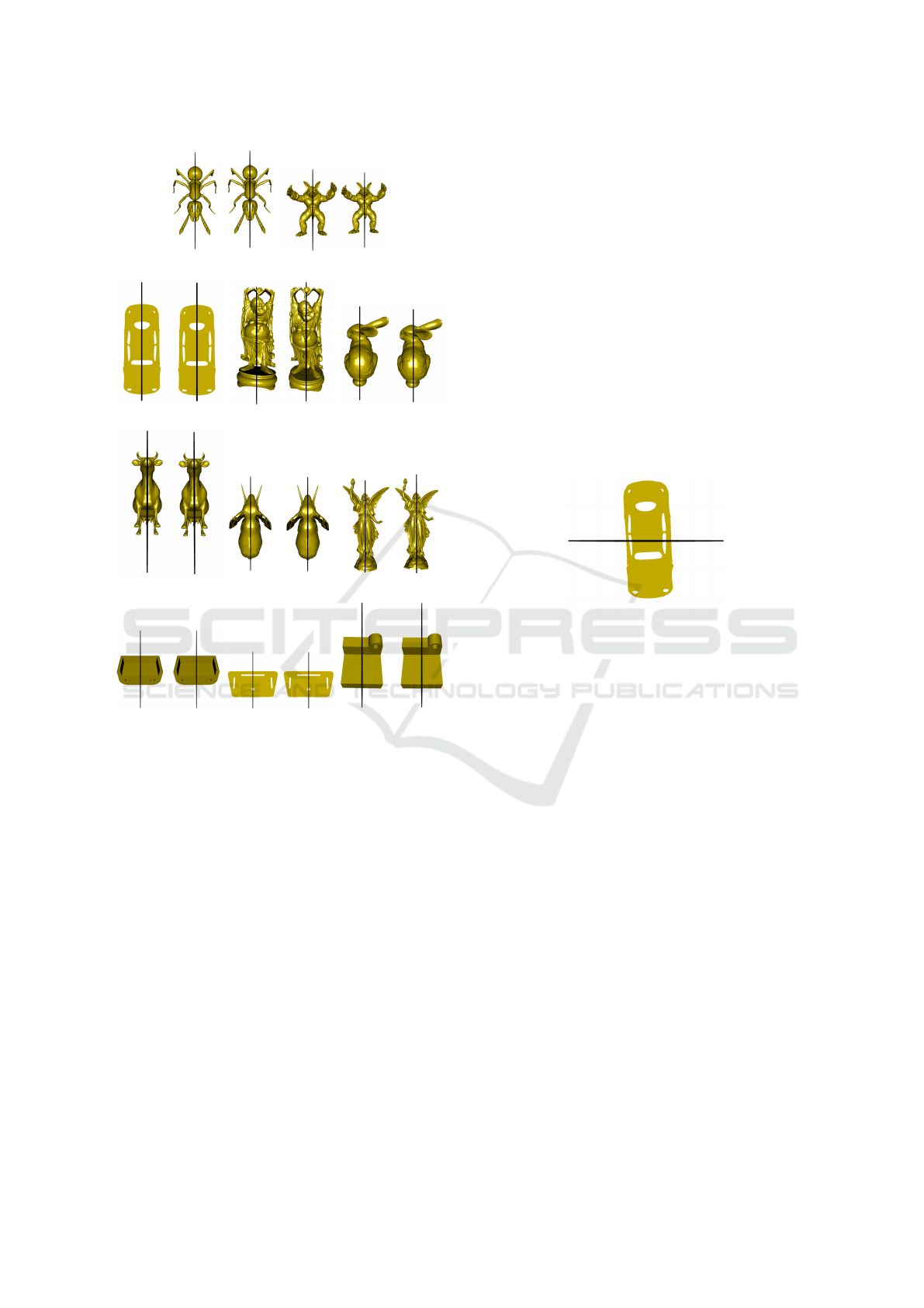
(a) Ant (b) Armadillo
(c) Beetle (d) Buddha (e) Bunny
(f) Cow (g) Elephant (h) Lucy
(i) Component1 (j) Component2 (k) Component3
Figure 2: Resulting symmetry planes for Table 1, left: sym-
metry plane by our method, right: the symmetry plane by
the Hruda et al. method (Hruda et al., 2021).
measure sym
rel
, the more symmetric the object is
with respect to the given plane. Since the planes
acquired using our method return smaller values of
sym
rel
, they are of worse quality than those computed
by Hruda et al. method. If the resulting planes are ex-
amined visually, they do not significantly differ from
each other. The results can be seen in Figure 2, with
symmetry planes found by our method on the left, and
the planes found by Hruda et al. method on the right.
For the Beetle model there is a noticeable differ-
ence in results if the parameter t
a
is set to lower value.
This result can be seen in Figure 3. The model has two
strong symmetries, for the horizontal plane, the value
of the symmetry measure is smaller, but the generated
symmetry candidates lie closer to each other. This
is caused by the distribution of the input points. If
the parameter is set higher, to t
a
= 0.6, the horizon-
tal planes are filtered out, and do not skew the results.
These results demonstrate the importance of the filter-
ing step. Similarly, to limit such cases, the weights in
the density computation step are computed.
Our method also works well for models with
sparser point sampling, such as the models Com-
ponent1, Component2 and Component3, where
the points of the mesh are situated near the cor-
ners and holes, with long edges between them. Our
method can also find prominent approximate sym-
metry planes, such as for the Bunny model, where
the body is symmetric with respect to one plane and
the head with respect to another, or the Lucy model.
To accelerate, our method exploits the similarities
between the generated candidates and uses a fast den-
sity computation. If we compare the average time for
the Hruda et al. method of 1188.45 ms and the aver-
age time our method of 801.18 ms, we can state that
our method is on average 1.48 times faster.
Figure 3: Result for the Beetle model if t
a
= 0.4 is used.
10 CONCLUSION
The described method successfully finds the approxi-
mate symmetry planes in point clouds, and works well
for various types of models. In terms of the relative
symmetry measure the resulting planes are weaker
symmetries than those of the Hruda et al. method, but
the results are visually similar, see Figure 2, and our
density based method is on average 1.48 times faster.
In the future, we aim to generalize the candidate
creation process, and modify the method to detect
different types of symmetries. We would also like
to extend the method so it can work with different
types of input, such as volumetric data, and exploit
the detected planes for data compression. The algo-
rithm could be further accelerated by computation of
weights w
i
on the GPU.
ACKNOWLEDGMENTS
This work was supported by the project 23-04622L,
Data compression paradigm based on omitting self-
evident information - COMPROMISE, of the Czech
Fast Approximate Symmetry Plane Computation as a Density Peak of Candidates
191

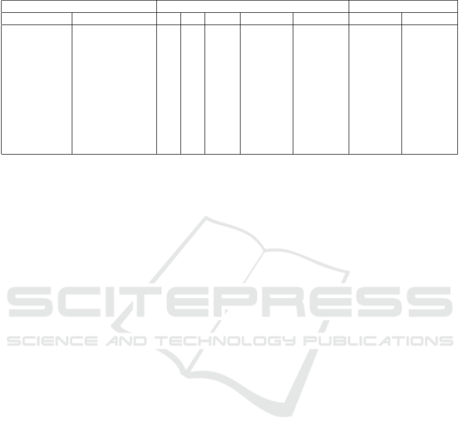
Table 1: Measured results of our density based method and the Hruda et al. method (Hruda et al., 2021).
Input Density peak method Hruda et al. method
Name Number of points t
a
D s
cell
sym
rel
Time [ms] sym
rel
Time [ms]
Ant 3495 0.4 25 0.1 0.8606616 820 0.9106182 1076
Armadillo 172974 0.5 50 0.05 0.5710908 1266 0.6171123 1680
Beetle 988 0.6 25 0.1 0.9107133 611 0.926909 856
Buddha 543103 0.6 25 0.08 0.4112466 1012 0.5553252 1186
Bunny 34834 0.4 25 0.05 0.4153833 1185 0.4667871 1115
Cow 2903 0.4 25 0.1 0.9133395 659 0.9134644 925
Elephant 19753 0.5 25 0.1 0.5669933 679 0.7926888 1032
Lucy 750001 0.6 25 0.05 0.4501815 1439 0.5110494 1877
Component1 1506 0.8 25 0.1 0.9787157 123 0.9789074 988
Component2 4302 0.8 25 0.1 0.9425972 913 0.9523025 1432
Component3 1410 0.8 25 0.1 0.7442631 106 0.7974733 906
Science Foundation, and by the Ministry of Educa-
tion, Youth and Sports under the Students Research
project SGS-2022-015.
REFERENCES
Cicconet, M., Hildebrand, D. G., and Elliott, H. (2017).
Finding mirror symmetry via registration and optimal
symmetric pairwise assignment of curves. 2017 IEEE
International Conference on Computer Vision Work-
shops (ICCVW).
Ecins, A., Fermuller, C., and Aloimonos, Y. (2017). Detect-
ing reflectional symmetries in 3d data through sym-
metrical fitting. 2017 IEEE International Confer-
ence on Computer Vision Workshops (ICCVW), page
1779–1783.
Fang, R., Godil, A., Li, X., and Wagan, A. (2008). A
new shape benchmark for 3d object retrieval. Lecture
Notes in Computer Science, page 381–392.
Gao, L., Zhang, L.-X., Meng, H.-Y., Ren, Y.-H., Lai, Y.-
K., and Kobbelt, L. (2021). Prs-net: Planar reflec-
tive symmetry detection net for 3d models. IEEE
Transactions on Visualization and Computer Graph-
ics, 27(6):3007–3018.
Gothandaraman, R., Jha, R., and Muthuswamy, S. (2020).
Reflectional and rotational symmetry detection of cad
models based on point cloud processing. 2020 IEEE
4th Conference on Information & Communication
Technology (CICT), 34:1–5.
Hruda, L., Dvo
ˇ
r
´
ak, J., and V
´
a
ˇ
sa, L. (2019). On evaluating
consensus in ransac surface registration. Computer
Graphics Forum, 38(5):175–186.
Hruda, L., Kolingerov
´
a, I., and V
´
a
ˇ
sa, L. (2021). Robust,
fast and flexible symmetry plane detection based on
differentiable symmetry measure. The Visual Com-
puter, 38(2):555–571.
Jacobson, A. (2024). Common 3d test models.
Ji, P. and Liu, X. (2019). A fast and efficient 3d reflection
symmetry detector based on neural networks. Multi-
media Tools and Applications, 78(24):35471–35492.
Kov
´
acs, E. (2012). Rotation about an arbitrary axis and re-
flection through an arbitrary plane. In Annales Math-
ematicae et Informaticae, pages 175–186.
Levoy, M., Gerth, J., Curless, B., and Pull, K. (2005). The
stanford 3d scanning repository.
Li, B., Johan, H., Ye, Y., and Lu, Y. (2016). Efficient 3d re-
flection symmetry detection: A view-based approach.
Graphical Models, 83:2–14.
Martinet, A., Soler, C., Holzschuch, N., and Sillion,
F. X. (2006). Accurate detection of symmetries
in 3d shapes. ACM Transactions on Graphics,
25(2):439–464.
Mitra, N. J., Guibas, L. J., and Pauly, M. (2006). Partial
and approximate symmetry detection for 3d geometry.
ACM SIGGRAPH 2006 Papers on - SIGGRAPH ’06,
page 560.
Mitra, N. J., Pauly, M., Wand, M., and Ceylan, D. (2013).
Symmetry in 3d geometry: Extraction and applica-
tions. Computer Graphics Forum, 32(6):1–23.
Nagar, R. and Raman, S. (2019). Detecting approximate re-
flection symmetry in a point set using optimization on
manifold. IEEE Transactions on Signal Processing,
67(6):1582–1595.
Shilane, P., Min, P., Kazhdan, M., and Funkhouser, T.
(2004). The princeton shape benchmark. Proceedings
Shape Modeling Applications, 2004., page 167–388.
Wendland, H. (1995). Piecewise polynomial, positive defi-
nite and compactly supported radial functions of mini-
mal degree. Advances in Computational Mathematics,
page 389–396.
Yianilos, P. N. (1993). Data structures and algorithms for
nearest neighbor search in general metric spaces. In
Proceedings of the Fourth Annual ACM-SIAM Sym-
posium on Discrete Algorithms, SODA ’93, page
311–321, USA. Society for Industrial and Applied
Mathematics.
GRAPP 2025 - 20th International Conference on Computer Graphics Theory and Applications
192