Comparison of Monolithic and Structural Decision Models Using the

Hamming Distance

Andrii Shekhovtsov

1,2 a

, Amirkia Raﬁei

3 b

and Wojciech Sałabun

1,2 c

National Institute of Telecommunications Szachowa 1, 04-894 Warsaw, Poland

West Pomeranian Univ. of Technology

Zołnierska 49, 71-210 Szczecin, Poland

Yildiz Technical University Davutpa¸sa St., Esenler, 34220 Istanbul, Turkey

Keywords:

Multi-Criteria Decision Making, COMET, MCDA, Expected Solution Point.

Abstract:

This study shows a simple yet effective approach to comparing decision models built using the Characteristic

Objects Method (COMET). The proposed approach is based on the Hamming Distance and its adaptation for

complex decision problems that involve structural division of the model. We demonstrate the simulation-based

proof-of-concept and then demonstrate the proposed approach to the case study of evaluating ten hydrogen

cars based on the information provided by the manufacturers. We compared six decision models created based

on the preferences of three decision makers expressed using Expected Solution Point (ESP) and Triad Support

algorithm. The results obtained provide, on the one hand, some useful insights into customers’ preferences

and expectations for hydrogen cars and, on the other hand, show the utilization of the proposed comparison

methodology.

1 INTRODUCTION

Multi-Criteria Decision Making (MCDM) is the do-

main of operational research that investigates com-

plex decision problems, which usually involve many

different criteria (Zavadskas and Turskis, 2011). In

case of complex problems, the decision maker can

turn to a vast choice of decision support methods,

from simple ones such as Technique for Order of

Preference by Similarity to Ideal Solution (TOPSIS)

(Li et al., 2023) or Stable Preference Ordering To-

wards Ideal Solution (SPOTIS) (Dezert et al., 2020),

to complex methods, such as Characteristic Objects

METhod (COMET) (Sałabun et al., 2019), which can

identify even complex decision maker’s preferences

in the complete domain of the decision problem.

The motivation for this study comes from the fact

that the COMET method and other pairwise compar-

ison methods lack a clear way to measure or compare

the results of different decision models. For example,

it may be necessary to include the opinions of mul-

tiple experts or to build several decision models and

use methods to combine their results (Dehe and Bam-

https://orcid.org/0000-0002-0834-2019

https://orcid.org/0009-0004-3490-550X

https://orcid.org/0000-0001-7076-2519

ford, 2015). In these cases, correlation measures can

help identify and understand differences between the

results of different methods or models (Yelmikheiev

and Norek, 2021). However, there is no simple way to

compare COMET models or predict how much their

results might differ, creating a gap in the tools avail-

able for decision-making analysis.

In this paper, we present a simple yet effective ap-

proach to measuring the differences between COMET

decision models, demonstrated by using the exam-

ple of hydrogen cars. In such a case study was cho-

sen, the use of MCDM methods has become essen-

tial with the increasing number of hydrogen-powered

alternatives available not only in the transportation

ﬁeld. Recently, there has been interest in research

in the MCDM ﬁeld in hydrogen technologies, such

as covering production, infrastructure, and transporta-

tion systems.

The main contribution of this paper is to show

an approach on how to compare decision models

based on the COMET model using the Hamming dis-

tance and how to adapt this approach to the structural

models. To demonstrate our proposed approach, we

present a simulation that shows that it is possible to

predict the outcome of the ranking comparisons based

on the Hamming distance between Matrices of Expert

Judgements for different models. We also present this

280

Shekhovtsov, A., Raﬁei, A. and Sałabun, W.

Comparison of Monolithic and Structural Decision Models Using the Hamming Distance.

DOI: 10.5220/0013120200003890

Paper published under CC license (CC BY-NC-ND 4.0)

In Proceedings of the 17th International Conference on Agents and Artiﬁcial Intelligence (ICAART 2025) - Volume 3, pages 280-287

ISBN: 978-989-758-737-5; ISSN: 2184-433X

approach in a real-life case study on the evaluation of

hydrogen cars.

The rest of the paper is structured as follows. In

Section 3, we brieﬂy present the methods and algo-

rithms used for this research. Next, in Section 4.1,

we present the proof of concept of the comparison of

COMET models using the Hamming distance, then in

Sections 4.2 and 4.3, we present the case study of hy-

drogen cars and a proposition for the comparison of

structural COMET models. Finally, in Section 5, we

summarize our ﬁndings and discuss the directions for

future works.

2 RELATED WORKS

The ﬁeld of MCDM has seen extensive research, pro-

viding a wide array of methods to assist decision-

makers in addressing complex multi-criteria prob-

lems. Well-established techniques such as TOPSIS

and the Analytic Hierarchy Process (AHP), along

with their various modiﬁcations, offer clear and efﬁ-

cient ranking mechanisms. However, more advanced

methods such as COMET are speciﬁcally designed

to capture and model intricate decision-maker pref-

erences. Despite the widespread application of these

methods, a signiﬁcant research gap persists in the

comparison of decision models, particularly in the

case of approaches such as COMET or AHP, which

are being increasingly used in emerging areas. In this

section, we provide an overview of selected related

works and the usage of the AHP and COMET meth-

ods in practical applications.

Panchal et al. applied the AHP to address the crit-

ical issue of slope failure along highways in hilly re-

gions (Panchal and Shrivastava, 2022). In their study,

they developed a landslide hazard map for a section of

National Highway 5, using various causative factors.

Each of these factors was further divided into sub-

factors, with weights assigned according to the AHP

methodology. It shows the need to investigate how to

effectively compare MCDM models, especially when

different model structures can lead to varying results.

To facilitate such comparisons, additional tools and

methodologies are needed to ensure robust evalua-

tions of model effectiveness across different scenar-

ios.

Several other studies emphasize the importance of

the AHP method in various domains, demonstrating

its utility while avoiding the issue of model struc-

ture sensitivity and the need for tools to compare

MCDM models effectively. Awad and Jung applied

AHP to prioritize sustainable urban regeneration fac-

tors in Dubai, identifying the urban environment, eco-

nomic, and social / cultural sectors as key elements.

Although their ﬁndings were insightful, they did not

address how the structure of their model could have

inﬂuenced the results, leaving this challenge unad-

dressed (Awad and Jung, 2022). Similarly, Ekmek-

cio

glu et al. used fuzzy AHP to create a district-

based ﬂood risk map for Istanbul, classifying land

use and storm return periods as the most signiﬁ-

cant factors, but also did not explore how different

model structures could impact the results (Ekmek-

cio

glu et al., 2021). Yariyan et al. combined FAHP-

ANN for earthquake vulnerability mapping in Iran,

achieving superior accuracy compared to traditional

AHP, but again without investigating how varying

structures could affect their ﬁndings (Yariyan et al.,

2020). These examples highlight the widespread use

of AHP in decision making, but also show that none

of these studies addresses the critical issue of compar-

ing models with different structures, underscoring the

need for more advanced tools to ﬁll this gap.

In current practice, the common approach to com-

paring MCDM methods typically involves analyz-

ing the results obtained from different methods and,

in some cases, applying distance metrics to assess

the similarities or differences between these results.

For example, Yelmikheiev and Norek compared the

COMET and TOPSIS methods for selecting optimal

vacuum cleaner robots based on criteria such as price,

engine power, and noise level. After ranking the al-

ternatives using both methods, they evaluated the re-

sults based on distance to the reference objects, show-

ing that the COMET method provided more accurate

results in their case (Yelmikheiev and Norek, 2021).

This highlights the utility of comparing results, but

also points to the limitations of relying solely on ﬁnal

rankings, because it does not offer a true model com-

parison, which should focus on comparing the entire

structure of the models rather than discrete points or

outputs.

Shekhovtsov et al. tackled a similar problem

by using three different MCDM methods to evalu-

ate preferences across a set of alternatives. They

tested the impact of varying the number of alternatives

and criteria on the ﬁnal rankings and then compared

the results using correlation coefﬁcients (Shekhovtsov

et al., 2021). Their ﬁndings indicated that the rank-

ings were very similar and that an increase in alter-

natives and criteria improved this similarity. Wi˛eck-

owski and Dobryakova also explored this compara-

tive approach, applying the COMET method to eval-

uate swimming athletes for sprint events (Wi˛eckowski

and Dobryakova, 2021). They reduced the complex-

ity of the problem by dividing the initial structure

and later compared the COMET results with other

Comparison of Monolithic and Structural Decision Models Using the Hamming Distance

281

MCDM methods using correlation metrics such as

Pearson and WS similarity coefﬁcients. A more com-

prehensive approach was presented by Sałabun et al.,

who conducted a broad simulation study to bench-

mark multiple MCDA methods (Sałabun et al., 2020).

Their research compared a variety of MCDA tech-

niques, including TOPSIS, VIKOR, COPRAS, and

PROMETHEE II, by evaluating their performance us-

ing different criteria, parameters, and ranking similar-

ity coefﬁcients such as Weighted Spearman correla-

tion and WS coefﬁcients. Through extensive simu-

lations, the study revealed how factors like the num-

ber of attributes, decision variants, and normalization

techniques inﬂuenced the ﬁnal rankings.

However, the current study builds on these efforts

by focusing on a more effective approach to com-

paring decision models identiﬁed through different

structures of the COMET method. Unlike previous

works that primarily evaluate ranking outcomes, this

study delves into the comparison of the entire struc-

ture of decision models. By shifting the focus from

merely comparing results to analyzing the underly-

ing model architectures within the COMET frame-

work, this research offers a deeper and more compre-

hensive understanding of the differences and similari-

ties between decision models identiﬁed using various

COMET structures.

3 PRELIMINARIES

In this section, we brieﬂy describe the methods and al-

gorithms used in this study. Each subsection contains

a short description of the method and related refer-

ences.

3.1 Characteristic Objects Method

(COMET)

The Characteristic Objects Method (COMET) distin-

guishes itself from other Multiple Criteria Decision

Analysis (MCDA) methods by being completely im-

mune to the ranking reversal phenomenon (Sałabun

et al., 2019). It makes it possible to develop a Multi-

Criteria Decision Analysis (MCDA) model that al-

ways provides unambiguous results, no matter how

much the alternative set changed (Kizielewicz et al.,

2021). The key points of the algorithm of the COMET

method are as follows:

Step 1. Deﬁne the Problem Space – Identify the crite-

ria for the decision problem and assign fuzzy numbers

to represent each criterion.

Step 2. Generate Characteristic Objects – Use the

Cartesian product of fuzzy numbers to create a set of

Characteristic Objects representing all possible com-

binations.

Step 3. Rank the Characteristic Objects – Perform

pairwise comparisons of the Characteristic Objects to

rank them based on expert judgment. Summarize the

judgments and calculate the preference values.

Step 4. Build the Rule Base – Convert each character-

istic object and its preference value into a fuzzy rule.

Step 5. Inference and Final Ranking – Use the fuzzy

rule base and Mamdani’s inference method to evalu-

ate and rank alternatives. Alternatives with a higher

preference value are better.

In Step 3. of the COMET method, the identiﬁed

pairwise comparison matrix contains only the values

{0, 0.5, 1} and deﬁnes the decision model. The re-

search gap lies in the fact that there are no studies

showing how to compare such models without calcu-

lating the ﬁnal results.

3.2 COMET Extensions

The main limitation of the COMET method is the

curse of dimensionality, which becomes a signiﬁ-

cant challenge when the method is applied to de-

cision problems involving a large number of crite-

ria. This issue arises because the number of pair-

wise comparisons required grows exponentially with

the number of criteria, making it impractical for large

problems. However, recent advancements in research

have addressed these limitations, making the COMET

method more applicable even when larger sets of cri-

teria are involved in the decision-making process.

One such advancement is the Expected Solution

Point (ESP) in COMET, which automates the pair-

wise comparison step. This automation is achieved by

allowing the decision maker to provide an ESP, from

which the Matrix of Expert Judgements (MEJ) is au-

tomatically generated. This innovation signiﬁcantly

reduces the decision maker’s workload and enhances

the efﬁciency of the model identiﬁcation process, as

shown in recent studies (Shekhovtsov et al., 2023).

Another approach to mitigating the complexity

of the COMET method is the Triad Support Algo-

rithm, which minimizes the number of pairwise com-

parisons required. The algorithm assumes that if the

expert judgments are consistent and free from errors,

the evaluations of characteristic objects should form

a transitive relationship. Using this property, the al-

gorithm reduces the need for redundant comparisons,

thereby streamlining the process of identifying the

MEJ matrix (Shekhovtsov and Sałabun, 2023).

Finally, the Structural COMET approach offers a

solution by breaking down a complex decision prob-

lem into several smaller submodels, which are then

ICAART 2025 - 17th International Conference on Agents and Artiﬁcial Intelligence

282

aggregated to form the ﬁnal decision model. This

method signiﬁcantly reduces the size of the MEJ ma-

trices, which in turn reduces the number of pairwise

comparisons needed to build the model. This struc-

tural model approach makes COMET more manage-

able for larger decision problems and has proven to be

an effective way to handle the curse of dimensionality

(Shekhovtsov et al., 2020).

These advancements collectively represent sub-

stantial progress in overcoming the limitations of the

COMET method, making it more suitable for decision

problems with a larger number of criteria, while pre-

serving the method’s strengths in capturing complex

preferences.

3.3 Weighted Spearman’s Coefﬁcient

The Weighted Spearman’s correlation coefﬁcient is

often used in the MCDM domain because of its use-

ful properties for the decision-making process. This

approach places a larger weight on the comparison in

the head of the rankings, which is usually more im-

portant to the decision maker. This is the main differ-

ence from the Spearman rank correlation coefﬁcient,

which has equal weights for all positions (Pinto da

Costa and Soares, 2005). Weighted Spearman’s cor-

relation coefﬁcient r

is deﬁned for two samples with

rank values x

and y

of size N as (1).

= 1−

∑

i=1

− y

)

((N − x

+ 1) + (N − y

+ 1))

+ N

− N

(1)

4 CASE STUDY

In this section, we ﬁrst show the proof of concept of

measuring the differences in MEJ matrices with nor-

malized Hamming distance using a simulation study,

and then we try to adapt the same approach to com-

plex structural models built for the evaluation of hy-

drogen cars.

4.1 Simulation Proof of Concept

The Hamming distance can be easily adapted to mea-

sure the differences between two different COMET

models expressed as MEJ matrices. Suppose that we

have two MEJ matrices of size N × N with elements

(1)

i j

and α

(2)

i j

, respectively. In this notation, the gen-

eral formula for the Hamming distance will take the

form of (2):

∑

i=1

∑

j=1

δ(α

(1)

i j

, α

(2)

i j

)

, (2)

where δ(α

(1)

i j

, α

(2)

i j

) is a special function equal to 1

only and only if x

and y

are different. In this way, the

Hamming distance provides a simple way to quantify

the differences between two MEJ matrices (Norouzi

et al., 2012).

We designed a simple simulation experiment to

check if there is any correlation between the Ham-

ming distance, which allows us to measure the dif-

ferences between models, and Weighted Spearman’s

correlation, which allows us to measure differences in

the resulting rankings. The single run of the simula-

tion can be described as follows:

1. Deﬁne the decision matrix X of a speciﬁc size.

2. Calculate two random ESP points esp1 and esp2

in the problem domain.

3. Identify two COMET models using generated

ESPs.

4. Calculate the Hamming distance between identi-

ﬁed models and save it for further analysis.

5. Calculate two rankings, one using the COMET

model deﬁned by esp1 and the other using

COMET deﬁned by esp2.

6. Calculate the correlation r

between these rank-

ings and save it for further analysis.

Notice that both the decision matrix values and the

ESP points values were generated from the uniform

random distribution in the range [0, 1).

We ran the simulation 1000 times for all combi-

nations of a number of criteria m ∈ {3, 4, 5, 6, 7} and

a number of alternatives m ∈ {10, 15, 20} to include

results for different decision matrix sizes. However,

all those results turn out to be very similar, and there-

fore, in Fig. 1, we present 15000 simulation runs to-

tal. The upper and right parts of this ﬁgure present

the distribution of the normalized Hamming distance

and the r

values, respectively. The middle part of

the ﬁgure presents the joint distribution of simulation

results. The black line determines the sigmoid func-

tion ﬁtted to the data. As can be seen, there is a cer-

tain dependency of r

value and Hamming distance

for monolithic models (e.g., the model with no sub-

models). It can be observed that we got lower simi-

larity in the results for those models for larger values

of the Hamming distance. To be sure that we will get

similar results, we need to have models that are dif-

ferent for no more than 0.1-0.15 Hamming distance.

Besides the fact that it is possible to get similar rank-

ings with models with a 0.4 distance value, it is much

more possible to obtain results that are uncorrelated or

even inverted. On the other side of the visualization,

there are a small number of examples when generated

Comparison of Monolithic and Structural Decision Models Using the Hamming Distance

283

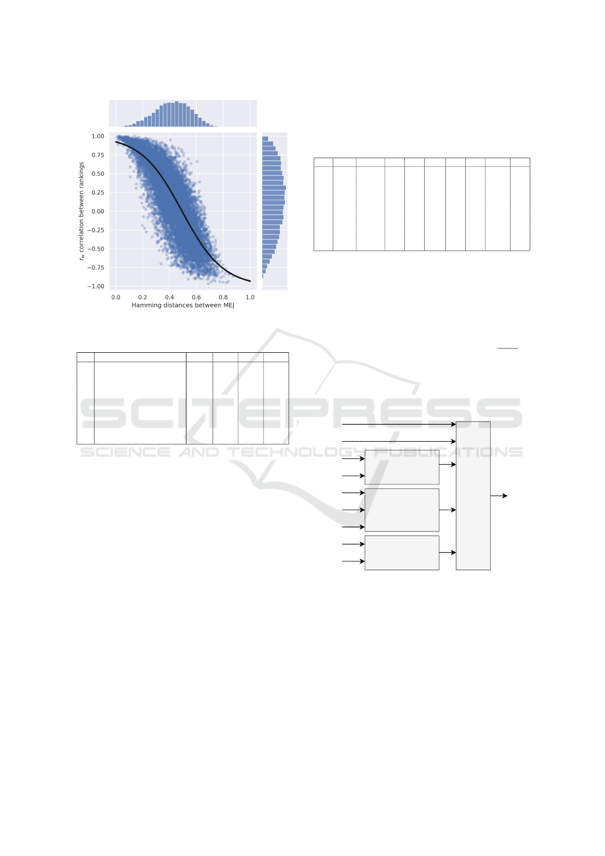
Figure 1: Simulation results.

Table 1: Criteria description.

Criteria names Units CV

Year – 2015 2022 2024

Estimated price $K 30 60 100

Range km 400 600 800

Power output KW 100 150 400

Hydrogen tank capacity kg 4.4 5.5 6

Horse power – 130 180 550

Max torque Nm 260 350 410

0 to 100 acceleration time s 4.5 8 12.5

Max speed km/h 130 170 250

COMET models have almost inverted MEJ (normal-

ized Hamming distance close to 1), and it is expected

that the resulted rankings for those models are almost

reversed (r

value close to -1). The Pearson r cor-

relation between those two vectors is approximately

−0.85, implying a negative correlation between those

variables.

4.2 Example of Hydrogen Cars

Evaluation

We present a case study of the evaluation of hydrogen

cars based on the following criteria: year of the start

of the production, approximated or estimated price,

range of the car, technical parameters of the engine,

tank capacity, acceleration and maximum speed. All

criteria are presented in Table 1 along with the mea-

surement units and characteristic values required to

create and identify the COMET model.

The data of the alternatives were manually col-

lected from the manufacturer’s websites during the

preliminary stage of the study, and the characteristic

values were selected based on the minimum, maxi-

mum, and median values of the collected alternatives.

The alternatives and the respective values of the crite-

ria are presented in Table 2.

Table 2: Alternatives’ data.

2023 50.00 646 128 5.60 182 406 9.20 161

2023 60.00 612 135 6.33 161 394 9.20 179

2021 59.00 579 103 5.46 174 299 9.00 165

2019 45.00 437 155 4.40 211 364 5.80 160

2022 30.00 400 150 4.40 134 260 7.80 130

2015 66.50 594 100 5.64 136 406 12.50 160

2024 90.00 504 295 6.00 401 347 6.00 180

2023 45.00 590 134 5.60 182 300 7.80 170

2022 68.00 800 220 5.43 300 347 6.50 200

2022 100.00 800 400 5.43 550 347 4.50 250

Each decision maker has their own preferences,

and therefore we need to identify personalized deci-

sion models using the COMET method. However,

if we try a straightforward approach to solving this

problem using this decision problem, we will fail

because of the dimensionality problem. The deci-

sion maker will need to compare t = 3

= 19683

characteristic objects, which will result in

t(t−1)

193, 700, 403 pairwise comparisons. However, as we

showed in Section 3, there are several methods to

drastically reduce the number of pairwise compar-

isons, namely the ESP-COMET approach, the Triad

Support algorithm, and the structural model approach.

Power Efficiency

Engine

Speed Performance

- Final model

Figure 2: Structural division of the problem.

Taking this into account, we ﬁrst divide our deci-

sion problem into four submodels, as shown in Fig.

2. This structure logically aggregates the criteria that

determine the power efﬁciency of the vehicle, engine

power, speed performance, and price and production

year in the ﬁnal model. Next, we asked three decision

makers E1, E2, and E3 for input to identify six deci-

sion models with this structure: Each decision maker

identiﬁes two models, one using the ESP-COMET ap-

proach and the other using the Triad Support algo-

rithm. Exemplary results of the identiﬁcation process

can be seen in Fig. 3, where three MEJ matrices iden-

ICAART 2025 - 17th International Conference on Agents and Artiﬁcial Intelligence

284

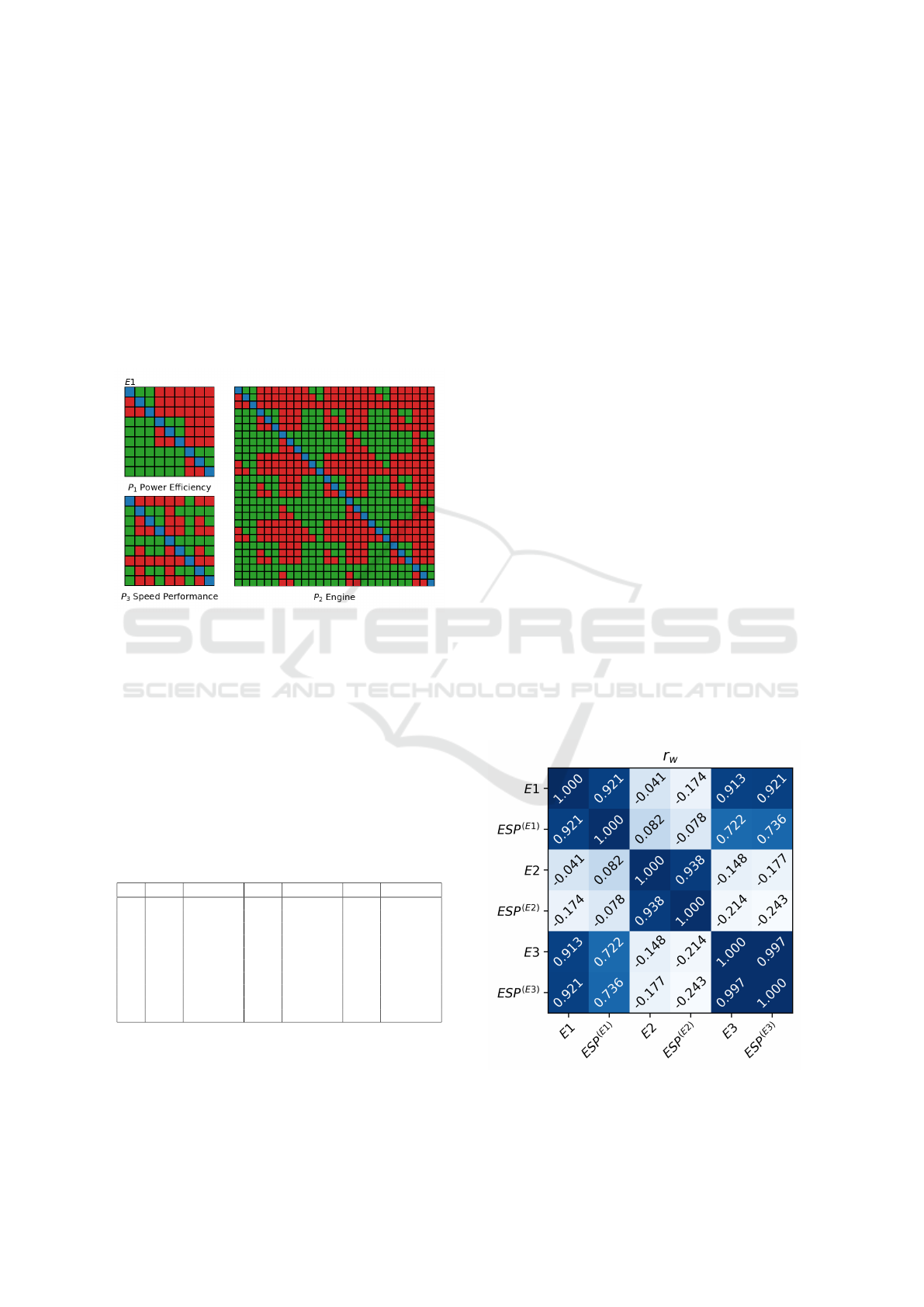
tiﬁed using the Triad Support algorithm are presented.

The ﬁnal model for each decision maker was automat-

ically calculated based on the importance weights of

the criteria provided by each of them. Using the ESP-

COMET approach does not require pairwise compari-

son and manual identiﬁcation. Usage of the structural

approach requires only 423 pairwise comparisons in-

stead of 193 million, which is more than 450 thousand

times less. However, the Triad Support algorithm pro-

vides an additional reduction, which depends on the

decision maker and, in the case of E1 (Fig. 3), results

in only 182 comparisons.

Figure 3: The MEJ matrices for submodels identiﬁed by

the ﬁrst expert with the help of Triad Support algorithm.

Green, blue and red values represent values 1, 0.5 and 0

respectively.

For the sake of shortness, we do not demonstrate

the rest of the models but present the resulting rank-

ings R

in Table 3 for the six identiﬁed models: E1,

ESP

(E1)

, E2, ESP

(E2)

, E3, ESP

(E3)

, where E j is a

model built using the Triad Support algorithm by j−th

decision maker and ESP

(E j)

is the model built using

the ESP-COMET approach using input from j−th de-

cision maker.

Table 3: Rankings obtained using all six models.

E1 R

ESP

(E1)

E2 R

ESP

(E2)

E3 R

ESP

(E3)

1 1 3 5 2 2

7 8 9 9 7 7

6 4 7 7 6 6

5 6 5 3 4 4

3 5 10 10 1 1

8 7 8 8 10 9

10 10 4 4 9 10

2 2 6 6 3 3

4 3 2 2 5 5

9 9 1 1 8 8

Table 3 contains the ranking for all identiﬁed mod-

els. As we can see, there are little differences between

E j and R

ESP

(E j)

rankings which are expected

behavior. For the E1, the most preferred alternative is

, and the least preferred is A

. Notice that the differ-

ences in rankings between the models identiﬁed man-

ually and automatically for E1 begin at the second po-

sition of the ranking. The most preferred alternative

for a second expert is A

0, which landed ninth and

eighth in other rankings. The second most preferred

alternative for E2 is A

, and the differences in these

rankings can be visible only at the 3rd and 5th posi-

tions. The rankings R

E3 and R

ESP

(E3)

are almost

the same, with only two last alternatives swapped. In

further investigation, we can see that the rankings cre-

ated using models from E1 and E3 are generally simi-

lar, but the rankings provided by the E2 models differ

signiﬁcantly.

The conclusions about the similarity of the rank-

ings are clearly visible in Fig. 4 where the heatmap

of Weighted Spearman’s r

correlation values is pre-

sented. As expected, we can see that the rankings pro-

vided by the models identiﬁed by the input of E j ex-

pert (e.g. E j and ESP

(E j)

) are similar. Between mod-

els of the expert E1 Weighted Spearman’s correlation

value is 0.92. This correlation is equal to 0.94 for E2

and 0.997 for E3. It proves the point that automatic

identiﬁcation using ESP can provide results that are

very similar to the manually identiﬁed models. The

rankings of the E1 models are generally similar to the

ranks obtained with E3 due to the similar preferences

of both experts. However, the correlation values of

the models E1 and E3 with models of E2 are close

to zero, which implies that these rankings have really

low correlation or are not correlated at all. This shows

that E2 has very different preferences from the other

two experts.

Figure 4: Weighted Spearman’s r

correlation values be-

tween all rankings (rounded up to 3 positions).

Comparison of Monolithic and Structural Decision Models Using the Hamming Distance

285

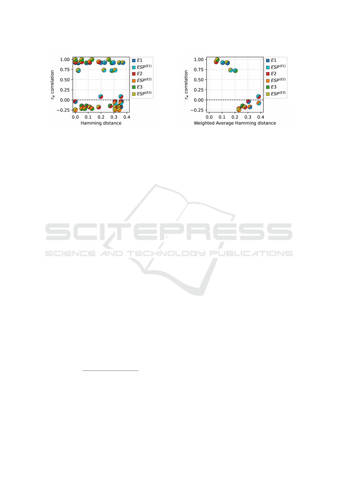
Figure 5: Relations between hamming distances between

MEJ and r

correlation between ﬁnal rankings for each sub-

models.

However, is it possible to predict the similarity

of the results on the basis of the similarity of the

models? To investigate this, we prepare the visual-

ization in Figure 5 in which each dot represents a

comparison between submodels for two different ex-

perts. For example, one of the dots is created by cal-

culating the Hamming distance between the P

sub-

model of E1 and the respective submodel of E3 and

Weighted Spearman’s correlation between ﬁnal rank-

ings of those two models (e.g., E1 and E3 models).

In this visualization, we can see that there is no easy

way to tell if we get high or low similarity in the re-

sults based on the Hamming distances between differ-

ent submodels.

4.3 Weighted Average Hamming

Distance

The simulation designed showed that there is a cor-

relation between the Hamming distance between two

different MEJ matrices and the r

correlation between

the ﬁnal ranking obtained using these two models in

the case of the monolithic model. However, the prob-

lem is less trivial if we need to compare structural

models. Therefore, we propose to use the Weighted

Average Normalized Hamming Distance d

w,H

, which

allows us to get a value that will aggregate all sub-

models. The weights should be determined based on

how many criteria are included in the speciﬁc sub-

model, and then the ﬁnal results should be divided by

the sum of weights to obtain the normalized values

(3).

w,H

· d

(MEJ

(1)

, MEJ

(2)

)

∑

i=1

, (3)

where w

is a weight for the i-th submodel,

(MEJ

(1)

, MEJ

(2)

) is the normalized Hamming dis-

tance between MEJ for the i-th submodels for two dif-

ferent experts calculated according to (2).

Figure 6: Relations between Weighted Average normal-

ized Hamming distance between MEJ and r

correlation

between results in different models.

Based on the structure of the problem 2, we can

assign the following weight vector: w = {2, 3, 2, 9}

for the set of submodels {P

, P

}, based on the

number of criteria aggregated using the model.

Next, we visualize the relation between the

Weighted Average Normalized Hamming distances

and the respective r

correlations in Figure 6. It can

be clearly seen that we can distinguish two clusters

with a Weighted Average Hamming distance lower

than or higher than 0.2. It can be seen that we obtain a

smaller distance and a higher similarity of results for

models identiﬁed toward similar preferences (that is,

rankings E1, E3, and ESP rankings for them, as well

as manual and ESP ranking for E2). However, if we

move to the combinations of other rankings with the

ranks identiﬁed based on the preferences of the expert

E3. Those models are more different, which can be

seen in the Weighted Average Normalized Hamming

distance values, and the ﬁnal rankings are slightly re-

versed or uncorrelated (based on the respective values

. It shows that we can predict to a certain point if

or not we will get similar results in terms of rankings

even for the structural model, even if there are no al-

ternatives or we don’t want to evaluate them.

5 CONCLUSIONS

In this paper, we propose a simple but effective so-

lution to approximate the differences in the results of

the identiﬁed COMET models. We also show how

to adapt this approach to a more complex structural

model and show its efﬁciency in the practical case

study of choosing a hydrogen car. In addition to that,

we show that the ESP-COMET approach can provide

results that can be obtained using the manual or triad-

supported identiﬁcation of the MEJ. This underlines

its usefulness in solving practical decision-making

problems, as this approach eliminated the pairwise

comparison step of model identiﬁcation, but allowed

ICAART 2025 - 17th International Conference on Agents and Artiﬁcial Intelligence

286

us to achieve a similar level of accuracy.

However, the work has some limitations that

should be addressed in future research. In addition

to the fact that the normalized Hamming distance and

the average normalized Hamming distance provide

satisfactory results in predicting r

values for both

monolithic and structural models, the precision of this

method can be higher and this fact should be investi-

gated in future work. This approach should also be

investigated in depth in other study cases to show its

practical applicability, as well as extended to a larger

sample of people, to better investigate differences in

models and preferences. There is also a possibility

to generalize the approach for other methods such as

AHP or Ranking Comparison (RANCOM) methods.

ACKNOWLEDGMENTS

The work was supported by the National Science Cen-

tre 2021/41/B/HS4/01296.

REFERENCES

Awad, J. and Jung, C. (2022). Extracting the planning ele-

ments for sustainable urban regeneration in dubai with

ahp (analytic hierarchy process). Sustainable Cities

and Society, 76:103496.

Dehe, B. and Bamford, D. (2015). Development, test

and comparison of two multiple criteria decision anal-

ysis (mcda) models: A case of healthcare infras-

tructure location. Expert Systems with Applications,

42(19):6717–6727.

Dezert, J., Tchamova, A., Han, D., and Tacnet, J.-M.

(2020). The spotis rank reversal free method for multi-

criteria decision-making support. In 2020 IEEE 23rd

International Conference on Information Fusion (FU-

SION), pages 1–8. IEEE.

Ekmekcio

glu, Ö., Koc, K., and Özger, M. (2021). District

based ﬂood risk assessment in istanbul using fuzzy an-

alytical hierarchy process. Stochastic Environmental

Research and Risk Assessment, 35:617–637.

Kizielewicz, B., Shekhovtsov, A., and Sałabun, W. (2021).

A new approach to eliminate rank reversal in the mcda

problems. In International Conference on Computa-

tional Science, pages 338–351. Springer.

Li, Y., Cai, Q., and Wei, G. (2023). Pt-topsis meth-

ods for multi-attribute group decision making under

single-valued neutrosophic sets. International Jour-

nal of Knowledge-based and Intelligent Engineering

Systems, (Preprint):1–18.

Norouzi, M., Fleet, D. J., and Salakhutdinov, R. R. (2012).

Hamming distance metric learning. Advances in neu-

ral information processing systems, 25.

Panchal, S. and Shrivastava, A. K. (2022). Landslide hazard

assessment using analytic hierarchy process (ahp): A

case study of national highway 5 in india. Ain Shams

Engineering Journal, 13(3):101626.

Pinto da Costa, J. and Soares, C. (2005). A weighted rank

measure of correlation. Australian & New Zealand

Journal of Statistics, 47(4):515–529.

Sałabun, W., Piegat, A., W˛atróbski, J., Karczmarczyk, A.,

and Jankowski, J. (2019). The comet method: the

ﬁrst mcda method completely resistant to rank rever-

sal paradox. European Working Group Series, 3.

Sałabun, W., W ˛atróbski, J., and Shekhovtsov, A. (2020).

Are mcda methods benchmarkable? a comparative

study of topsis, vikor, copras, and promethee ii meth-

ods. Symmetry, 12(9):1549.

Shekhovtsov, A., Kizielewicz, B., and Sałabun, W. (2023).

Advancing individual decision-making: An extension

of the characteristic objects method using expected so-

lution point. Information Sciences, 647:119456.

Shekhovtsov, A., Kołodziejczyk, J., and Sałabun, W.

(2020). Fuzzy model identiﬁcation using monolithic

and structured approaches in decision problems with

partially incomplete data. Symmetry, 12(9):1541.

Shekhovtsov, A. and Sałabun, W. (2023). The new algo-

rithm for effective reducing the number of pairwise

comparisons in the decision support methods. pages

243–254.

Shekhovtsov, A., Wi˛eckowski, J., and W ˛atróbski, J. (2021).

Toward reliability in the mcda rankings: Comparison

of distance-based methods. In Intelligent Decision

Technologies: Proceedings of the 13th KES-IDT 2021

Conference, pages 321–329. Springer.

Wi˛eckowski, J. and Dobryakova, L. (2021). A fuzzy as-

sessment model for freestyle swimmers - a compar-

ative analysis of the mcda methods. Procedia Com-

puter Science, 192:4148–4157. Knowledge-Based

and Intelligent Information & Engineering Systems:

Proceedings of the 25th International Conference

KES2021.

Yariyan, P., Zabihi, H., Wolf, I. D., Karami, M., and

Amiriyan, S. (2020). Earthquake risk assessment us-

ing an integrated fuzzy analytic hierarchy process with

artiﬁcial neural networks based on gis: A case study

of sanandaj in iran. International Journal of Disaster

Risk Reduction, 50:101705.

Yelmikheiev, M. and Norek, T. (2021). Comparison of

mcda methods based on distance to reference objects-

a simple study case. Procedia Computer Science,

192:4972–4979.

Zavadskas, E. K. and Turskis, Z. (2011). Multiple criteria

decision making (mcdm) methods in economics: an

overview. Technological and economic development

of economy, 17(2):397–427.

Comparison of Monolithic and Structural Decision Models Using the Hamming Distance

287