Finding the Shear Reﬂection Symmetry Plane in a 3D Point Cloud

ıtek Po

1 a

, Ivana Kolingerov

1 b

and Damjan Strnad

2 c

Department of Computer Science and Engineering, University of West Bohemia,

Technick

a 8, 306 14 Plze

n, Czech Republic

Department of Computer Science, Faculty of Electrical Engineering and Computer Science, University of Maribor,

Koro

ska cesta 46, 2000 Maribor, Slovenia

Keywords:

Symmetry, Reﬂection, Shearing, Computer Graphics.

Abstract:

Many objects, namely man-made ones, show signs of various types of symmetry. The most common type

perceived by humans is reﬂection symmetry to some plane. When detecting the symmetry for geometric

models, the existing algorithms look for orthogonal reﬂection symmetry. However, the models can be sheared,

therefore, algorithms detecting shear reﬂection symmetry would be useful. In this paper, we propose an

algorithm for detecting the plane of shear reﬂection symmetry in a 3D point cloud on condition that the shear

was done in one of the coordinate axes.

1 INTRODUCTION

Symmetry is a distinctive visual feature of geometric

objects, enabling their faster human understanding.

Mathematically, it is typically deﬁned as a geomet-

ric transformation different from the identity, map-

ping the object into itself. The most often used trans-

formation is planar reﬂection, mirroring the object

by a plane of symmetry, and many methods for its

computer detection have been developed. However,

the used reﬂection is orthogonal, although managing

more general directions of reﬂection could be useful

to handle objects that are symmetric in a more general

sense, e.g., an object and its skewed copy.

When detecting the plane of symmetry for com-

puter geometric models, we work with approximate

symmetry, since we cannot rely on perfect symmetry

in real 3D data. Therefore, it is reasonable to propose

symmetry detection algorithms that work with noisy

or incomplete data.

This paper makes the ﬁrst step to handling one

variant of non-orthogonal reﬂection symmetry, a

shear reﬂection symmetry. The proposed algorithm

handles 3D point clouds, possibly noisy or incom-

plete, sampled from the surface of a geometric object.

The input data are supposed to have been sheared in

the x-direction, by an unknown angle. The output is

https://orcid.org/0009-0004-4489-2837

https://orcid.org/0000-0003-4556-2771

https://orcid.org/0000-0003-4468-0290

the best ﬁtting plane of shear reﬂection symmetry and

the shear angle to the x-axis.

1.1 Background

The perfect symmetry of the given 3D points of an ob-

ject X can be understood as a geometric transforma-

tion T such that T (X) = X, i.e., the object X is invari-

ant to the transformation T . The approximate sym-

metry can then be understood as a geometric transfor-

mation T such that T (X) approximately matches X.

A common type of symmetry is reﬂection symme-

try, where the transformation T is a reﬂection over a

given plane. Let the plane be described by the signed

distance from the origin d and the normal vector n.

Then the orthogonal reﬂection of the point p onto its

image r through the plane (n, d) is given by

r = p − 2 ∗ (dot(n, p)− d) ∗ n, (1)

where dot is the scalar product of two vectors.

Naturally or artiﬁcially skewed data can be de-

scribed by an afﬁne transformation that shifts each

point in a certain direction by the value of its distance

from a given line parallel to that direction. This trans-

formation is often called shear mapping, shear trans-

formation or just shearing. The equation of the gen-

eral afﬁne transformation, mapping the source vector

x = [x, y, z]

by the transformation matrix A into the

destination vector x

′

= [x

′

, y

′

, z

′

]

, is as follows:

′

= Ax. (2)

Poór, V., Kolingerová, I. and Strnad, D.

Finding the Shear Reﬂection Symmetry Plane in a 3D Point Cloud.

DOI: 10.5220/0013120400003912

Paper published under CC license (CC BY-NC-ND 4.0)

In Proceedings of the 20th International Joint Conference on Computer Vision, Imaging and Computer Graphics Theory and Applications (VISIGRAPP 2025) - Volume 1: GRAPP, HUCAPP

and IVAPP, pages 203-210

ISBN: 978-989-758-728-3; ISSN: 2184-4321

203

In 3D space, shearing can be done in three di-

rections. The corresponding transformation matrices

have the following forms:

shearing in x−direction : A =





1 0 0

a 1 0

b 0 1





, (3)

shearing in y−direction : A =





1 a 0

0 1 0

0 b 1





, (4)

shearing in z −direction : A =





1 0 a

0 1 b

0 0 1





, (5)

where a and b are coefﬁcients of the shear; shearing in

the x-direction affects all axes except the x-axis, etc.

It is possible to assemble shearing in more axes, how-

ever, in this work, only the shear matrix (4) is used

and, what is more, b = 0.

The coefﬁcients are derived from the angle at

which the object is sheared. We call this angle the

shear angle and the coefﬁcients are its tangent. For ex-

ample, if the object is to be sheared in the y-direction

at an angle of 45° only due to the inﬂuence of the

x-axis, then the matrix (4) with the coefﬁcients a =

tan(45) and b = 0.

1.2 Related Work

Symmetry detection is widely studied in various ﬁelds

including compression (Simari et al., 2006), object re-

construction (Sipiran, 2017) and alignment (Chaouch

and Verroust-Blondet, 2009), re-meshing (Podolak

et al., 2007), symmetrical editing (Martinet et al.,

2006), facial image analysis (Mitra and Liu, 2004).

Due to the importance of this topic, various types of

symmetry were addressed, such as perfect, approxi-

mate, global, local, extrinsic, intrinsic, rotational, and

reﬂection; the detection methods operate namely on

images and 3D points. An overview is provided in

(Mitra et al., 2013).

As reﬂection symmetry is the most important,

there are many methods for its detection. Most of

them have some limitations; e.g., they detect only

planes passing through a reference point (for exam-

ple, the object centroid) (Sun and Sherrah, 1997; Mar-

tinet et al., 2006; Li et al., 2016). These methods are

suitable for determining the global symmetry of the

entire object but not its local symmetry where dif-

ferent reference points are needed. The method in

(Schiebener et al., 2016) does not have this limita-

tion and is thus suitable also for local symmetry but

additional knowledge is needed, such as the position

from which the object is scanned. A similar method

is (Ji and Liu, 2019), which needs an additional neu-

ral network training dataset. There are a few methods

that impose no limitations on the input data, such as

in (Hruda et al., 2022).

Shear is indirectly used in the search for symme-

try in images, as the projective transformation dis-

torts the objects in the scene and they appear skewed.

Several algorithms have been presented to solve this

problem, e.g., (Gross and Boult, 1994; Bruckstein and

Shaked, 1998; Friedberg, 1986; Cham and Cipolla,

1995). These algorithms are based on the extraction

of features from the shape and either take into account

the entire contour and are insensitive to noise, or con-

sider locally deﬁned characteristic features; it brings

instability and sensitivity to noise.

As far as we know, there is no direct method for

shear symmetry in a 3D point cloud. However, meth-

ods for object registration can be applied - we can

see symmetry detection as a special case of registra-

tion where both input objects are the same. Among

the registration algorithms, there are also speciﬁc al-

gorithms for afﬁne transformations (Ji et al., 2017;

Shu et al., 2021). However, these algorithms need

a proper adjustment so that their output is a detected

plane of symmetry and they are unnecessarily com-

plex for solving the symmetry detection problem.

Our work focuses on global, approximate, shear

reﬂection symmetry in a 3D point cloud, sampled

from the surface of the object. For easier understand-

ing, the algorithm is ﬁrst described in a simpliﬁed ver-

sion, for a ﬁxed shear angle, in Section 2. An ex-

tension of the algorithm for an arbitrary shear angle

is presented in Section 3. The limitation of the al-

gorithm is that only shear along the x-axis is taken

into account. The case of an unknown shear direction

could be solved by triple repetition of the algorithm.

However, a general shear in a more complicated direc-

tion, combined from transformations in more axes, is

out of scope of the algorithm. Such shears are compli-

cated even to be perceived correctly and they are am-

biguous in the sense that the results could have been

achieved by more than one series of transformations.

2 THE SIMPLIFIED

ALGORITHM FOR A FIXED

SHEAR ANGLE

The input of the algorithm is a set of 3D points from

the surface of an object, the output is the equation of

the plane of shear symmetry together with the shear

angle. A plane (n, d) is described by its normal n

GRAPP 2025 - 20th International Conference on Computer Graphics Theory and Applications

204

and its distance d from the origin. The shear angle

tells us the angle of transformation of the shear object

in a certain direction (compared to the untransformed

object). The version of the algorithm presented in this

section works with a ﬁxed direction and angle (i.e.,

the ﬁxed shear angle is the same as the shear angle

at the output). The shear reﬂection symmetry plane

detection algorithm is composed of three main steps:

1. Generating orthogonal and shear planes,

2. Evaluation of all planes,

3. Selection of the best plane.

A detailed description of the algorithm steps is be-

yond the scope of this text.

2.1 Generating Planes

Planes are generated directly from the input point

cloud. All pairs of points are processed, and each

pair generates two planes. Let the points p and q

be the currently processed pair of points. The ﬁrst

plane reﬂects orthogonally the point p to the point q

(see Equation 1). We need this plane for cases where

the detected reﬂection symmetry plane is not sheared.

The second plane, called the shear plane, reﬂects at a

shear angle. In addition, the input of the algorithm

contains the shear vector shear, the ﬁrst two com-

ponents of which indicate the shear direction and the

third component the shear angle.

Shear reﬂection through the original plane is

achieved by constructing an auxiliary plane whose

normal vector ns is in the direction of the input vector

shear and its distance from the origin is determined

by the distance of the intersection x of the original

plane with the line constructed by the input point p

and the ns direction (see Fig. 1). The term original

plane refers to the plane currently being processed by

the algorithm.

Figure 1: An example of constructing an auxiliary plane to

achieve shear reﬂection.

2.2 Evaluation of all Planes

The next step of the algorithm is the evaluation of the

generated planes. For each plane, the evaluation is

based on the distances of the mirrored points from the

original points. First, a plane is constructed from the

auxiliary vector, and then a measure is evaluated for

it. This evaluation process is performed for all points

of the input set over all generated planes. The overall

evaluation of one plane is given by the sum of partial

evaluations.

Finally, the partial evaluation of the given plane

for one given point from the input set of points is cal-

culated. Through the shear plane constructed as de-

scribed in the previous text, the point p is reﬂected

to the point r orthogonally via Equation 1. From the

thus reﬂected point r, the distances of all points of the

input set are calculated. The partial evaluation of the

input plane for the input point p is calculated by the

function minimum which returns the minimum value

from the distances of all points to point p.

2.3 Selection of the Best Plane

The selection of the plane with the best evaluation is

done by the ascending rating of the resulting evalua-

tions associated with the planes. The plane with the

lowest rating is taken as the best. In other words, the

mirror of points obtained by shear reﬂection through

the given plane has the smallest distance of points

from the original points.

However, the algorithm can return more planes

since it has the entire list of evaluated planes at its

disposal. More planes than one may be desirable for

objects where the plane of symmetry is not clearly

visible to humans. Such a selection is then made by

the user, who must take into account the value of the

evaluation.

2.4 Optimization

The proposed algorithm has been so far explained as

brute force. To achieve a reasonable runtime, various

optimization techniques can and should be incorpo-

rated. One of the techniques with the biggest impact

is input data reduction. A 3D spatial grid with a ﬁxed

cell size is built over the input data points. All points

in individual cells are then averaged. The points cre-

ated in this way are then used in the next steps of the

algorithm. The number of points is directly propor-

tional to the number of grid cells. The input points

are normalized to a cube of unit edge and shifted so

that the centroid of the object is at the origin of the

world coordinate system.

Finding the Shear Reﬂection Symmetry Plane in a 3D Point Cloud

205

The biggest bottleneck of the algorithm is the eval-

uation of the planes. Optimization is done both to

reduce the set of planes to be evaluated and for the

evaluation itself. One can imagine that the gener-

ated planes in the ﬁrst step are many, especially for

large data sets. As part of this step, the conditions for

adding a new plane to an existing data structure are

established. The distance of the plane from the origin

and the deviation of the direction of the normal from

the ﬁxed directions are veriﬁed. Assuming that the

resulting plane passes through the origin (or its small

neighborhood), we keep only planes with the distance

from the origin smaller than the chosen threshold e

Similarly, we can also limit the normal direction of

the plane, with a known shear it is likely that the re-

sulting plane will be somewhere within the angle e

from the direction of shear or the orientation of world

coordinates.

Another signiﬁcant optimization is performed in

the evaluation of planes. The experiments show that a

lot of time is devoted to the evaluation of planes that

end up with a worse measure than the best planes.

Since the resulting measure of one plane is given as

the sum of partial measures of all points, it is possi-

ble to terminate the evaluation process of the current

plane on the base of additional knowledge, such as the

best evaluation received so far.

3 THE FULL ALGORITHM FOR

AN ARBITRARY SHEAR

ANGLE

The algorithm described so far worked with addi-

tional knowledge of the shear angle (obtained at the

input of the algorithm). This section describes a gen-

eralization of the algorithm by removing the limita-

tion of a previously known shear angle. Thus, the

required input of the algorithm is only a set of 3D

points. The current limitation of the algorithm to the

x-axis remains.

3.1 The Proposed Extension

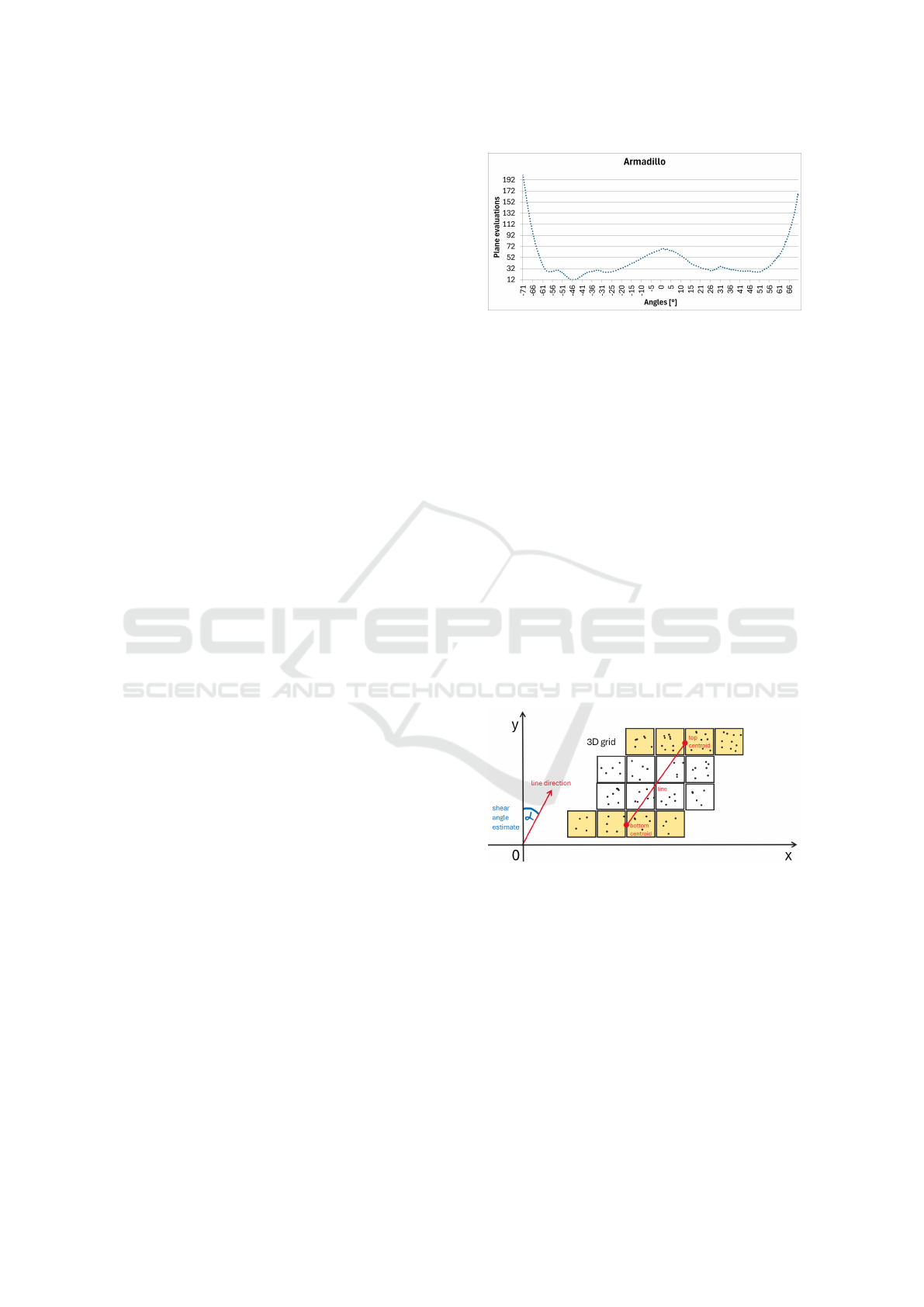
The problem of ﬁnding an unknown shear angle in

one axis corresponds to the problem of ﬁnding an

extreme in the graph of plane evaluations as a func-

tion of shear angle, see an example in Figure 2. For

time reasons, we want to avoid the computation of

this graph and still ﬁnd the extreme. In order to avoid

computation in the entire interval of angles, an initial

estimate of the shear angle is needed.

Figure 2: Planes evaluation for various shear angles over the

Armadillo object. Microsoft Excel was used as the graph

generator.

3.2 Shear Angle Estimation

One can imagine the estimate of the shear angle as the

angle between the y-axis and a straight line dividing

the object vertically in two when projected onto the

xy-plane. The straightforward approach is the use of a

pre-created 3D grid. In particular, it concerns the base

and ceiling cells. From these two sets of cells, two

points are determined as the centroids of the points

contained in these sets. These two points construct

a straight line that passes through the object. When

projecting such a straight line into 2D (xy-plane in our

case), the angle between the straight line and the y-

axis indicates the skew of the grid. This angle is also

the desired estimate. A schematic is shown in Figure

3, with an example on a real data set shown in Figure

4. The estimate is then used to construct an initial

interval for ﬁnding the resulting shear angle.

Figure 3: Sketch of the shear angle estimation construction

process based on the bottom and top points of the 3D grid

cells. For simplicity, projection to the xy-plane is used.

3.3 Finding Shear Angle in Interval

With a known estimate of the shear angle, the search

of the optimum can be limited to only a small sub-

interval of angles. First, a total of ﬁve values are de-

termined, from which the search sub-interval is then

constructed. The ﬁve values are a set formed around

the estimate. For the estimate α

and for the neigh-

borhood coefﬁcient b, the set is composed as

GRAPP 2025 - 20th International Conference on Computer Graphics Theory and Applications

206

Figure 4: Shear angle estimate on the Lion data with the an-

gle estimate (red line) and the plane found by the algorithm

(black line). For simplicity, only the bottom and top cells

of the 3D grid are shown, which are used to calculate the

centroids and construct the line.

{−(2∗b)+α

, −b+α

, α

+b, α

+(b∗2)}. (6)

Subsequently, a measure is calculated for these

ﬁve values using our detection algorithm. A search

sub-interval is constructed from the two values with

the best measure. This process is repeated for −α

At the end, a total of two search sub-intervals are

available, one for a positive estimate and one for a

negative estimate. A binary search is used over these

two intervals. The two best obtained values are com-

pared and the best value is declared as the resulting

shear angle.

4 EXPERIMENTS AND RESULTS

First, in Section 4.1, the basic experiments and results

for the simpliﬁed proposed method with a ﬁxed shear

angle are presented. These experiments focus on the

correctness of the resulting plane and the calculation

time. Further in Section 4.2 there are experiments and

results for the extended method of ﬁnding the shear

angle. Here, the main subject is comparing the results

of the extended method against the best possible ones

obtained from previous experiments.

4.1 Experiments and Results for

Simpliﬁed Method

Figure 5 shows objects with their sheared symmetry

planes detected by the proposed method. Objects are

displayed so that the detected plane (indicated by a

line) is perpendicular to the plane of projection. They

were taken from various datasets (Fang et al., 2008;

Levoy et al., 2005; Shilane et al., 2004). The re-

sults except for Bunny look correct in visual inspec-

tion. More detailed analysis is beyond the scope of

this text.

Since we do not know of another method for shear

symmetry detection, we cannot perform a comparison

and instead compare the best detected shear symme-

try plane with the best detected reﬂection symmetry

plane that is obtained for un-sheared data. We mainly

experimented with the plane evaluation measurement

across different angles and the algorithm run time.

As a reference method for the detection of orthog-

onal symmetry, we have chosen (Hruda et al., 2020).

This method does not require additional information

for input data. As an experiment, we took the out-

put of the reference method for an object that was not

sheared. Then we sheared the result plane accord-

ing to the best angle obtained by our algorithm. We

obtained the best shear angle by re-running our algo-

rithm for angles ranging from −90 to 90 degrees with

the step equal to 0.1 and selecting the best result. The

comparison is based on the angle difference between

our detected plane and the plane additionally sheared

according to our obtained shear angle. Table 1 shows

the results for all objects. The biggest difference can

be seen with the Bunny object. This is mainly due to

the selection of the best angle.

If we detect a shear symmetry plane in the data,

where we know the shear angle, then we can assume

that the detected plane will be sheared at an angle op-

posite to the angle of the sheared data. We performed

an experiment that detects a shear plane with different

ﬁxed shear angles for one speciﬁc object, Armadillo

(see Figure 5 (b)), sheared in the x-axis at an angle

of 45 degrees. Figure 2 shows the results of individ-

ual measurement values for different angles (a smaller

value is better). One can see that the best evaluation

is around an angle of −45 degrees, which was the as-

sumption of the experiment.

Computation time for the tested objects can be

seen in Table 2. Different sizes of simpliﬁcation de-

pending on the total number of points are determined

by the chosen simpliﬁcation algorithm and the shape

of the object.

4.2 Experiments and Results for

Proposed Method

Table 3 compares the best obtained shear angle (as

in Table 1) with the shear angle found using the ex-

tended algorithm. Data is generated for every single

instance of the Armadillo object (see Figure 5 (b)) that

has been sheared over the interval (-60, 60). Only a

few representative samples were selected.

Table 4 summarizes the error rate statistics of the

proposed algorithm extension compared to the best

found values. This experiment extends the previous

Table 3 by all previously used objects.

Finding the Shear Reﬂection Symmetry Plane in a 3D Point Cloud

207

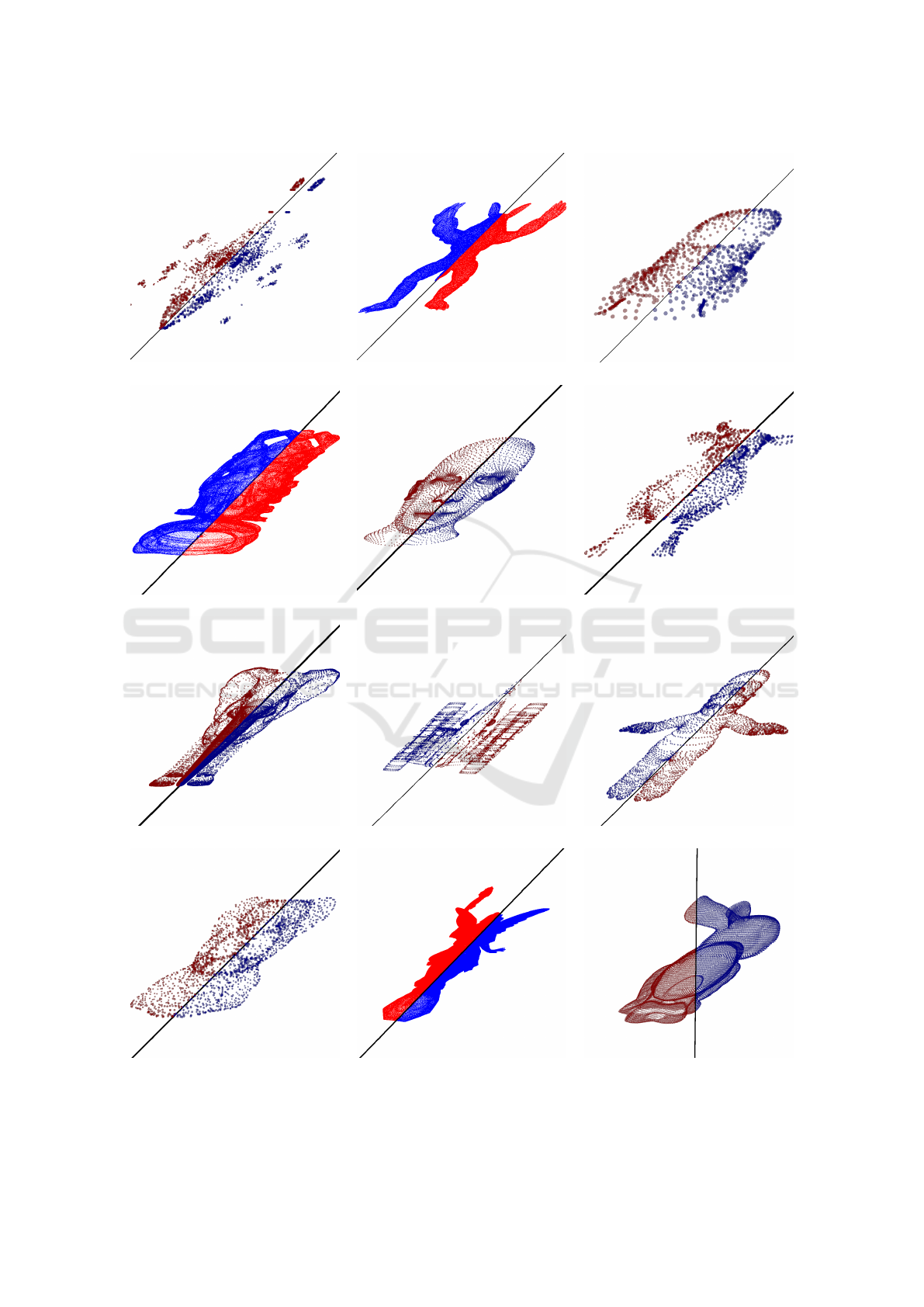
(a) Ant - 3495 (b) Armadillo - 172 974 (c) Beetle - 988

(d) Buddha - 543 103 Mannequin - 6737 (e) Cow - 2903 (f)

(g) Elephant - 19 753 (h) Formula - 10 969 (i) Homer - 5103

(j) Lion - 2213 (k) Lucy - 750 001 (i) Bunny - 34 834

Figure 5: Several objects with their symmetry planes detected using the proposed method. The number indicates the number

of 3D points in the point cloud.

GRAPP 2025 - 20th International Conference on Computer Graphics Theory and Applications

208

Table 1: Comparison of angle differences between the plane normals of the reference method and the proposed method. The

reference plane is sheared according to the best angle we obtained. Then both shear planes are compared. The distance from

the origin d is not shown as the compared planes pass through the centroid of the object.

Object

Reference Shear Reference Resulting Angle

plane Angle [°] Shear Plane Plane Diff. [°]

Ant (1.00, 0.00, 0.01) 44.9 (0.71, -0.70, 0.00) (-0.71, 0.71, -0.01) 0.60

Armadillo (1.00, 0.00, 0.01) 45.5 (0.70, -0.71, 0.00) (0.70, -0.71, 0.00) 0.21

Beetle (1.00, 0.00, 0.01) 45.1 (0.71, -0.70, 0.00) (0.71, -0.71, 0.00) 0.19

Buddha (-1.00, 0.00, 0.00) 44.5 (-0.71, 0.70, 0.00) (0.71, -0.70, 0.00) 0.18

Bunny (-0.99, 0.01, 0.17) 29.6 (-0.84, 0.49, 0.23) (1.00, -0.01, -0.01) 32.26

Cow (-1.00, 0.01, 0.01) 45 (-0.70, 0.71, 0.01) (-0.70, 0.72, 0.01) 0.31

Elephant (1.00, 0.00, -0.01) 45.1 (0.71, -0.71, 0.00) (-0.71, 0.71, 0.01) 0.58

Formula (1.00, -0.01, 0.00) 44.4 (0.71, -0.70, 0.00) (0.71, -0.71, 0.00) 0.17

Homer (-1.00, -0.01, -0.02) 45 (-0.71, 0.70, -0.02) (0.71, -0.70, 0.00) 1.32

Lion (1.00, -0.01, 0.00) 44.9 (0.70, -0.71, 0.00) (-0.71, 0.71, -0.01) 0.63

Lucy (-1.00, -0.04, 0.03) 45.5 (-0.73, 0.69, 0.04) (-0.72, 0.69, 0.01) 1.91

Mannequin (-1.00, 0.00, 0.00) 44.9 (-0.71, 0.71, 0.00) (-0.71, 0.71, 0.00) 0.28

Table 2: Computation time for one ﬁxed shear angle over

all objects. Times are measured for simpliﬁed objects.

Object Points

Points

(simpl.)

Time

[ms]

Ant 3495 162 508

Armadillo 172 974 281 1376

Beetle 988 283 1569

Buddha 543 103 361 2661

Bunny 34 834 342 2253

Cow 2903 253 1217

Elephant 19 753 272 1260

Formula 10 969 372 2981

Homer 5103 335 2389

Lion 2213 305 1797

Lucy 750 001 247 1301

Man-

nequin

6737 315 2012

5 CONCLUSION AND FUTURE

WORK

We proposed a new method for the detection of shear

reﬂection symmetry planes. We veriﬁed the method

on a set of objects. Currently, the method works with

shearing in one direction of the x-axis. Another limi-

tation is the chosen level of simpliﬁcation of the input

point cloud, which has a direct impact on the result

and calculation. Future work will focus on removing

the limitation to include an adaptive choice of point

cloud simpliﬁcation level such that the smallest pos-

sible data still gives correct results. At the same time,

another interesting challenge for future work is the

limitation of the ﬁxed shearing axis direction.

Table 3: Comparison between the best obtained shear angle

and the found shear angle for the Armadillo object. The

individual data angles represent the partial shear instances

of the Armadillo object.

Data

Angle

Shear

Angle

[°]

Found

Shear

Angle

[°]

Angle

Diff. [°]

-59 58.0 58.5 00.5

-50 49.0 46.9 02.1

-40 40.0 38.6 01.4

-30 29.0 29.4 00.4

-20 19.0 19.3 00.3

-10 09.0 09.3 00.3

0 00.0 -00.4 00.4

10 -11.0 -11.2 00.2

20 -21.0 -21.0 00.0

30 -31.0 -30.5 00.5

40 -41.0 -40.4 00.6

50 -51.0 -51.1 00.1

59 -60.0 -59.6 00.4

ACKNOWLEDGEMENTS

This research was supported by the Czech Science

Foundation under research project 21-08009K, the

Slovene Research and Innovation Agency under re-

search project N2-0181, Research Programme P2-

0041; V. Po

or was also supported by the Ministry of

Education, Youth and Sports under the Students Re-

search project SGS-2022-015.

Finding the Shear Reﬂection Symmetry Plane in a 3D Point Cloud

209

Table 4: Summary statistic error rate over all instances of the used models over the interval (-60, 60). The acquisition error

rate is based on the experiment in Table 3, i.e. the difference between the best obtained angle and the found angle over the

shear data interval.

Object Min. Diff. [°] Max. Diff. [°] Avg. Diff. [°] Med. Diff. [°]

Ant 0.00 1.00 0.25 0.00

Armadillo 0.00 3.40 0.54 0.40

Beetle 0.00 1.40 0.45 0.30

Buddha 0.00 6.10 0.99 0.50

Bunny 0.00 4.60 0.79 0.50

Cow 0.00 3.50 0.43 0.40

Elephant 0.00 1.00 0.25 0.10

Formula 0.00 2.40 0.53 0.40

Homer 0.00 2.00 0.32 0.20

Lion 0.00 1.80 0.50 0.40

Lucy 0.00 3.50 0.60 0.50

Mannequin 0.00 1.50 0.40 0.40

REFERENCES

Bruckstein, A. M. and Shaked, D. (1998). Skew-symmetry

detection via invariant signatures. Pattern Recogni-

tion, 31(2):181–192.

Cham, T.-J. and Cipolla, R. (1995). Symmetry detection

through local skewed symmetries. Image and Vision

Computing, 13(5):439–450.

Chaouch, M. and Verroust-Blondet, A. (2009). Alignment

of 3d models. Graphical Models, 71(2):63–76.

Fang, R., Godil, A., Li, X., and Wagan, A. (2008). A new

shape benchmark for 3d object retrieval. In Interna-

tional Symposium on Visual Computing, pages 381–

392. Springer.

Friedberg, S. A. (1986). Finding axes of skewed symme-

try. Comput. Vision Graphics Image Process., 34:138–

155.

Gross, A. D. and Boult, T. E. (1994). Analyzing skewed

symmetries. Int. J. Comput. Vision, 13:91–111.

Hruda, L., Kolingerov

a, I., and V

sa, L. (2020). Robust, fast

and ﬂexible symmetry plane detection based on differ-

entiable symmetry measure: Supplementary material.

Available at http://meshcompression.org/tvcj-2020.

Hruda, L., Kolingerov

a, I., and V

sa, L. (2022). Robust, fast

and ﬂexible symmetry plane detection based on differ-

entiable symmetry measure. Visual Comput., 38:555–

571.

Ji, P. and Liu, X. (2019). A fast and efﬁcient 3d reﬂection

symmetry detector based on neural networks. Multi-

media Tools and Applications, 78(24):35471–35492.

Ji, S., Ren, Y., Ji, Z., Liu, X., and Hong, X. (2017). An im-

proved method for registration of point cloud. Optik,

140:451–458.

Levoy, M., Gerth, J., Curless, B., and Pull, K. (2005).

The stanford 3d scanning repository. Available at

http://www.graphics.stanford.edu/data/3Dscanrep/.

Li, B., Johan, H., Ye, Y., and Lu, Y. (2016). Efﬁcient 3d re-

ﬂection symmetry detection: A view-based approach.

Graphical Models, 83:2–14.

Martinet, A., Soler, C., Holzschuch, N., and Sillion,

F. X. (2006). Accurate detection of symmetries in

3d shapes. ACM Transactions on Graphics (TOG),

25(2):439–464.

Mitra, N. J., Pauly, M., Wand, M., and Ceylan, D. (2013).

Symmetry in 3d geometry: Extraction and applica-

tions. Computer Graphics Forum, 32(6):1–23.

Mitra, S. and Liu, Y. (2004). Local facial asymmetry for

expression classiﬁcation. In CVPR.

Podolak, J., Golovinskiy, A., and Rusinkiewicz, S. (2007).

Symmetry-enhanced remeshing of surfaces. In Pro-

ceedings of the Fifth Eurographics Symposium on Ge-

ometry Processing (SGP ’07), pages 235–242. Euro-

graphics Association.

Schiebener, D., Schmidt, A., Vahrenkamp, N., and As-

four, T. (2016). Heuristic 3d object shape completion

based on symmetry and scene context. In Intelligent

Robots and Systems (IROS), 2016 IEEE/RSJ Interna-

tional Conference on, pages 74–81. IEEE.

Shilane, P., Min, P., Kazhdan, M., and Funkhouser, T.

(2004). The princeton shape benchmark. In Shape

Modeling Applications, 2004. Proceedings, pages

167–178. IEEE.

Shu, Q., He, X., Wang, C., Yang, Y., and Cui, Z. (2021).

Fast point cloud registration in multidirectional afﬁne

transformation. Optik, 229:165884.

Simari, P., Kalogerakis, E., and Singh, K. (2006). Fold-

ing meshes: Hierarchical mesh segmentation based on

planar symmetry. In Symposium on Geometry Pro-

cessing, volume 256, pages 111–119.

Sipiran, I. (2017). Analysis of partial axial symmetry on 3d

surfaces and its application in the restoration of cul-

tural heritage objects. In Proceedings of the IEEE

International Conference on Computer Vision Work-

shops, pages 2925–2933.

Sun, C. and Sherrah, J. (1997). 3d symmetry detection

using the extended gaussian image. IEEE Transac-

tions on Pattern Analysis and Machine Intelligence,

19(2):164–168.

GRAPP 2025 - 20th International Conference on Computer Graphics Theory and Applications

210