An Innovative Urban Delivery System Based on Customer-Selected
Addresses and Cost-Effective Driver Rates
Oualid Benbrik
1 a
, Rachid Benmansour
1,2 b
and Raca Todosijevi
´
c
2 c
1
Research Laboratory in Information Systems, Intelligent Systems and Mathematical Modeling, National Institute of
Statistics and Applied Economics, Rabat, Morocco
2
LAMIH CNRS UMR 8201, INSA Hauts-de-France, Polytechnic University of Hauts-de-France (UPHF),
Campus Mont Houy, F-59313 Valenciennes Cedex 9, France
Keywords:
Routing, City Logistics, Last-Mile, Crowd-Shipping, Optimization.
Abstract:
Last-mile delivery is undergoing rapid transformation due to the surge in home delivery services and the in-
creasing demand for convenience, driven by the digitalization of businesses. In response to this evolving
landscape, businesses are exploring innovative delivery methods, including the use of parcel lockers and drone
delivery. This study investigates a novel approach to last-mile delivery, utilizing non-professional delivery
personnel (crowd-shippers) to fulfill customer orders at designated addresses. By leveraging crowd-shippers
and considering service locations alongside a comprehensive set of drivers’ preferences—including familiarity
with the delivery area, traffic conditions, and ease of access— our aim is to minimize unsuccessful delivery
attempts, reduce costs, and align with environmental and societal sustainability goals. The main objective is
to minimize the total cost of delivery, accounting for both the total distance traveled and the drivers’ prefer-
ences regarding delivery points. We develop and solve a mixed-integer programming model that represents
this scenario, providing insights into the advantages of integrating drivers’ preferences into last-mile delivery
optimization strategies.
1 INTRODUCTION AND
LITERATURE REVIEW
The field of logistics encompasses various sub-areas,
each with distinct characteristics. Urban logistics, a
subset, focuses specifically on the challenges and op-
portunities related to managing the flow of goods in
urban environments. Its primary goal is to optimize
the supply chain in urban areas, emphasizing efficient
goods delivery, especially during the last mile, which
is a crucial aspect of urban logistics, referring to the
final phase of delivery, from the distribution cen-
ter to the end consumer. Last-mile delivery (LMD)
is the final stage of the distribution process, where
the shipment is transported from the last distribution
hub—such as a warehouse or distribution center—to
the recipient, whether at their home or at a nearby
collection point. This process is gaining momentum
due to the exponential growth of e-commerce (Tilk
a
https://orcid.org/0009-0009-3404-4136
b
https://orcid.org/0000-0003-2553-4116
c
https://orcid.org/0000-0002-9321-3464
et al., 2021) and urbanization (Amaral and Cunha,
2020). This urbanization trend is projected to increase
the urban population by almost 600 million by 2030,
reaching 5.2 billion , and further to 9.7 billion by
2050 (United Nations, Department of Economic and
Social Affairs, Population Division, 2022). This surge
in urban population emphasizes the need for effec-
tive last-mile solutions to meet the growing demand
for delivery services. However, it also presents chal-
lenges such as environmental impact, high costs, ser-
vice quality, and returns management ((Kiba-Janiak
et al., 2021),(Pahwa and Jaller, 2022)). In the first
quarter of 2023 in Morocco, merchant sites and Inter-
bank Electronic Payment Center (CMI) affiliates wit-
nessed substantial growth in online payment transac-
tions, totaling 2.9 billion dirhams (or a 32.3% increase
compared to the same period in 2022). Recently, in
early 2021, Amazon launched a challenge, in collab-
oration with the Massachusetts Institute of Technol-
ogy’s (MIT) Center for Transportation & Logistics,
which aimed to improve the efficiency of freight de-
livery by integrating driver expertise into optimization
models. Three research teams won a total of $175,000
Benbrik, O., Benmansour, R. and Todosijevi
´
c, R.
An Innovative Urban Delivery System Based on Customer-Selected Addresses and Cost-Effective Driver Rates.
DOI: 10.5220/0013120700003893
Paper published under CC license (CC BY-NC-ND 4.0)
In Proceedings of the 14th International Conference on Operations Research and Enterprise Systems (ICORES 2025), pages 229-238
ISBN: 978-989-758-732-0; ISSN: 2184-4372
Proceedings Copyright © 2025 by SCITEPRESS – Science and Technology Publications, Lda.
229

in prize money for their innovative route optimization
models in the Amazon LMD Research Challenge.
In light of these advancements, the main objec-
tive of this study, conducted as part of a research
project on logistics and urban mobility, is to address
the need for optimizing the LMD Problem (LMDP)
with consideration for service options and drivers’
preferences.
The Vehicle Routing Problem (VRP) and its var-
ious extensions have garnered significant attention in
academic literature. Foundational texts such as (Toth
and Vigo, 2002), (Golden et al., 2008), and (Toth and
Vigo, 2014) provide comprehensive insights into the
topic, while extensive literature reviews can be found
in works like (Cordeau et al., 2002), (Eksioglu et al.,
2009), (Laporte, 2009), and (Vidal et al., 2020).
The initial studies addressing both location and
routing dimensions can be traced back to the 1960s,
with notable contributions from authors such as
(Von Boventer, 1961), (Webb, 1968), and (Watson-
Gandy and Dohrn, 1973). Since then, a diverse ar-
ray of problems has emerged, each integrating routing
and location decisions, as highlighted in the survey by
(Prodhon and Prins, 2014). More recent works have
explored variations like the Swap-Body VRP (SB-
VRP), where trucks and semi-trailers are used to min-
imize total costs while managing complex constraints
related to customer accessibility and vehicle type (To-
dosijevi
´
c et al., 2017). Similarly, VRPs have been ap-
plied in logistics contexts involving truck scheduling,
where the goal is to optimize outbound deliveries by
minimizing total operation time, as seen in (Benman-
sour et al., 2024), which focuses on dispatching trucks
from a central terminal to serve dispersed customers
efficiently.
As society evolves toward a shared economy,
the role of Occasional Drivers (ODs) in crowdship-
ping is anticipated to become increasingly prominent
in future delivery systems. In crowdshipping, in-
dividual ODs operate as resource providers in the
sharing economy, offering their vehicles and time
to assist with LMD tasks, as discussed in (Strulak-
W
´
ojcikiewicz and Wagner, 2021). It is noteworthy
that many companies have integrated crowdshipping
into their business models since 2011, a trend signifi-
cantly accelerated by Amazon’s involvement starting
in 2015 (Jazemi et al., 2023). A key advancement in
this area is the introduction of the VRP with Occa-
sional Drivers (VRPOD) by (Archetti et al., 2016).
This variant combines traditional vehicle resources
with the capabilities of ODs, exploring various com-
pensation schemes to enhance operational efficiency.
The findings from (Archetti et al., 2016) indicate that
incorporating crowdshipping systems can yield more
effective delivery solutions. Further developments in
VRPOD include the work of (Macrina et al., 2017),
which added time window considerations, resulting
in the VRPOD with Time Windows and Multiple De-
liveries (VRPODTWmd). This version requires that
each customer be associated with specific time frames
for receiving packages, allowing ODs to execute mul-
tiple deliveries in a single trip. While some stud-
ies have concentrated on drivers’ behavior and their
willingness to serve as crowd-shippers (e.g., (Al Hla
et al., 2019)), others have adopted innovative method-
ologies. For instance, (Torres et al., 2022b) pro-
posed a two-stage stochastic framework to address a
stochastic variant of VRPOD, acknowledging uncer-
tainties in ODs’ availability. Their model addresses
the challenges associated with deliveries requiring
customer signatures, which may necessitate return-
ing items to the depot. The authors implemented a
branch-and-price algorithm to solve the problem pre-
cisely, alongside a column generation heuristic for
larger instances. Moreover, (Torres et al., 2022a)
introduced a framework wherein the destinations of
ODs are not predetermined. They modeled route du-
ration constraints to enhance ODs’ willingness to ac-
cept delivery routes, aiming to keep them manage-
able. This extension of their previous model (Torres
et al., 2022b) focused on minimizing both fixed and
variable compensations paid to ODs and employed
branch-and-price algorithms as well as rapid heuris-
tics for handling larger datasets.
The concept of the VRP with Delivery Op-
tions (VRPDO) has also emerged over the past two
decades, gaining traction in LMD optimization. This
problem extends traditional vehicle routing models by
considering various delivery options available to cus-
tomers, such as multiple delivery locations or pref-
erences regarding timing. The pioneering work of
(Cardeneo, 2005) first addressed the challenge of ac-
commodating multiple potential delivery addresses
within the VRPDO framework. Recently, (Tilk et al.,
2021) tackled the VRPDO, allowing shipments to be
directed to alternative locations with varying time
windows while also factoring in customers’ prefer-
ences for different delivery options. They proposed a
branch-price-and-cut algorithm to solve this complex
optimization issue. Delivery to optional points has
rapidly gained popularity in the realm of LMD, driven
by customers’ desire for timely and reliable service.
Customers can provide multiple potential delivery
points along with time windows, enabling the deliv-
ery plan to select the most suitable option. Earlier re-
search often overlooked customer preferences regard-
ing delivery locations (e.g., (Anily, 1996)), whereas
more recent studies have expanded the scope to in-
ICORES 2025 - 14th International Conference on Operations Research and Enterprise Systems
230

clude customer preferences in route planning (e.g.,
(Pourmohammadreza and Jokar, 2023)).
In an effort to balance route cost minimization
with customer satisfaction, which increasingly de-
mands flexibility in product delivery, (Los et al.,
2018) introduced a Generalized Pick-up and Deliv-
ery Problem (GPDP) that incorporates Time Win-
dows and Preferences (GPDPTWP). Their evalua-
tions demonstrated a 30% improvement in objective
function values through the use of both exact and ap-
proximate methods. Following this, (Dragomir et al.,
2022) explored the PDP with alternative locations and
overlapping time windows, seeking to optimize trans-
portation requests with a fleet of vehicles. They con-
sidered multiple pickup and delivery locations, in-
cluding alternate recipients, and assessed the feasibil-
ity of utilizing 24-hour locker boxes. Their solution
approach involved a multi-start adaptive large neigh-
borhood search with problem-specific operators. For
a comprehensive overview of VRPs specifically re-
lated to LMD in urban contexts, refer to (Jazemi et al.,
2023).
This paper introduces a variant of the VRPDO
that incorporates an additional constraint: Drivers’
Preferences. The study focuses on drivers’ prefer-
ences, considering multiple factors that influence the
assignment of delivery routes. Rather than relying
solely on distance, the model incorporates a broader
range of driver-related preferences, which are cap-
tured through the parameter β (see Section 2.1 for a
detailed explanation). By accounting for these fac-
tors, the model aims to enhance the efficiency of LMD
operations. This approach improves service qual-
ity by optimizing routes based on practical prefer-
ences, ensuring deliveries are carried out under more
favorable conditions for the drivers. To the best of
our knowledge, this study is the first to address the
LMDP while simultaneously considering both service
options and a comprehensive set of driver preferences
(cf. (Jazemi et al., 2023)). The primary objective is
to address practical challenges in online item deliver-
ies, particularly for customers requiring multiple de-
liveries within the same day, by ensuring that drivers’
routes are optimized for both efficiency and quality.
This is achieved by incorporating drivers’ preferences
into the routing process, thereby improving both ser-
vice performance and delivery conditions.
The main contributions of this paper are as fol-
lows:
• We propose a novel Mixed Integer Program-
ming (MIP) formulation designed to address the
LMDP. Our model incorporates service options
and drivers’ preferences, offering a new perspec-
tive on optimizing LMD with non-professional
delivery personnel (crowd-shippers).
• We extend the traditional LMD framework by ex-
plicitly considering drivers’ preferences related to
minimizing travel distance. This innovative ap-
proach aims to reduce delivery costs and increase
efficiency by aligning drivers’ preferences with
route optimization.
• We provide a comprehensive numerical analysis
of our proposed model, demonstrating its prac-
tical effectiveness through computational exper-
iments, with results achieved within reasonable
computing times.
The remaining sections of this paper are organized
as follows. Section 2 formally presents the problem
addressed in this study and provides an illustrative ex-
ample of a feasible solution. Section 3 introduces a
novel MIP model developed for solving the problem.
Experimental results of the MIP formulation are in-
vestigated in Section 4. Finally, Section 5 concludes
the paper by summarizing the findings and discussing
future perspectives.
2 PROBLEM DESCRIPTION
This section provides a comprehensive overview of
the LMDP with service options and drivers’ prefer-
ences. The first part formally describes the problem,
while the second part presents an illustrative example
to demonstrate a feasible solution to the problem.
2.1 Formal Problem Definition
We consider a central depot, denoted by index 1, from
which all deliveries originate. In an urban area, there
is a set of clients N = {2, 3, . . . , n}, each of whom
must be served from the depot. For each client i ∈ N ,
two potential delivery locations are available: a pri-
mary address (e.g., home) and an alternative address
(e.g., work), and the delivery must occur at one of
these suitable locations. Additionally, there is a set
V of m delivery vehicles responsible for complet-
ing these deliveries. The central depot, the main ad-
dresses, and the alternative addresses constitute a set
of nodes denoted by Ω. The main and alternative ad-
dress of client i (2 ≤ i ≤ n) are represented by the pair
of nodes (i, i + n − 1).
The delivery route planner aims to minimize the
parcel provider’s costs by assigning each driver to
clients in a way that aligns with their preferences.
In this model, the parameter β
k,i
plays a crucial role
in capturing the drivers’ preferences, allowing the
provider to optimize the assignment of delivery points
An Innovative Urban Delivery System Based on Customer-Selected Addresses and Cost-Effective Driver Rates
231

Table 1: Notations.
Sets and Indices
m number of vehicles available
n number of nodes representing the depot and the main addresses of customers
n
′
number of clients (n
′
= n − 1)
V set of vehicles available (1, 2, . . . , k, . . . , m)
N set of clients main location ( 2, 3, . . . , i, . . . , n)
Ω set of nodes (1, 2, . . . , 2n −1)
Parameters
d
i, j
distance between node i and node j
α
k
the price to be paid to the driver of vehicle k for each distance unit
β
k,i
the price to be paid for each delivery of vehicle k to serve node i
Decision variable
x
i, j,k
binary variable that equals 1 if vehicle k goes from node i to node j. 0 otherwise
y
k,i
binary variable that equals 1 if node i is served by the vehicle k ∈ V . 0 otherwise
u
i
positive integer variable representing the sequencing of nodes
while maintaining efficiency. Specifically, β
k,i
repre-
sents the cost incurred when the driver of vehicle k
serves client i. This cost takes into account various
parameters, such as the driver’s familiarity with the
neighborhood where client i is located, the ease of
circulation in that area (traffic density, terrain slope,
road conditions, etc.), as well as the proximity to the
driver’s workplace. Thus, the more these factors in-
crease the complexity of the delivery, the higher the
cost β
k,i
, indicating a lower preference for assigning
this client to the driver of vehicle k. This frame-
work captures a real-world scenario where the man-
ager prefers routes that minimize the overall travel
distance while respecting drivers’ preferences by aim-
ing for minimal operational costs. This is further fa-
cilitated by delivery flexibility, as each customer has
two addresses instead of just one. Moreover, the pa-
rameter α
k
is used to denote the payment to the driver
of vehicle k for each unit of distance traveled. Al-
though α
k
does not directly influence driver prefer-
ences, it ensures compensation for actual travel dis-
tances, offering a financial incentive for efficient rout-
ing aligned with those preferences. It is essential to
clarify that the terms vehicle k and driver k are used
interchangeably in this paper.
In practice, the items ordered online are gener-
ally small in size, allowing non-professional drivers to
manage deliveries using their own modes of transport,
which should ideally be environmentally friendly in
an urban setting. As the day begins, all items and
delivery vehicles are gathered at the depot, ready for
distribution. The items designated for delivery have
been prepared and packaged in advance, often the
day before, particularly considering that they were or-
dered online. Each vehicle k ∈ V must make a de-
livery tour, starting from node 1 and traversing a set
of clients, including their primary or alternative ad-
dresses. The distance between two consecutive nodes
i and j visited by the same delivery vehicle k is de-
noted as d
i, j
. Upon completing their delivery routes,
vehicles return to the depot, a step essential for overall
operational efficiency. This allows for the collection
of delivery receipts or signed documents from clients
for record-keeping and compliance. Additionally, the
return provides a centralized point for managing the
process, ensuring deliveries are tracked and crowd-
shippers are prepared for the next round. Addition-
ally, we assume, without loss of generality, that each
client i must be delivered to either their main address
or their alternate address by a single delivery vehi-
cle. Furthermore, we assume that time windows are
not considered and that the capacity of each vehicle is
sufficiently large, given the small size of the products
typically ordered online.
The primary objective is to minimize the total cost
of delivery, which includes the distance traveled by
vehicles, as well as considerations related to drivers’
preferences for more efficient route assignments. This
includes factors such as familiarity with the area, traf-
fic conditions, and so on. The problem is denoted as
LMDP-SODP, where SODP stands for Service Op-
tions and Drivers’ Preferences. The main notations
used to describe the problem are listed in Table 1.
2.2 Illustrative Example
The Figure 1 illustrates a feasible solution for LMDP-
SODP. It shows the routes of three different vehicles,
ICORES 2025 - 14th International Conference on Operations Research and Enterprise Systems
232

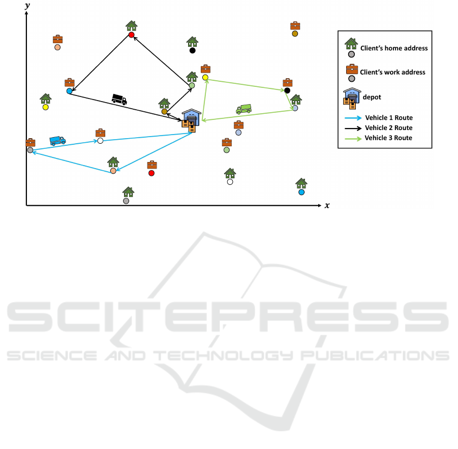
Figure 1: Illustration of a feasible solution to the LMDP-SODP with n
′
= 10 and m = 3.
each represented by a different color, starting from the
depot and visiting 10 clients. Each client is depicted
with two possible delivery locations: one for the home
address and one for the work address, and the vehicles
are assigned to visit one of these addresses based on
the model optimization criteria. The figure visually
demonstrates how each vehicle is routed to minimize
total delivery cost by considering various factors, in-
cluding drivers’ distance-based preferences, familiar-
ity with the area, traffic conditions, ease of access to
delivery locations, and so on.
3 MATHEMATICAL
FORMULATION
This section introduces a novel MIP formulation, tai-
lored for addressing the LMDP-SODP. The problem
can be formulated as a VRP that incorporates alterna-
tive locations and drivers’ preferences.
The delivery route planner must decide on optimal
routes for delivery vehicles that satisfy all constraints
while minimizing total cost.
3.1 Objective Function
min
∑
k∈V

∑
i∈Ω
∑
j∈Ω
i̸= j
α
k
d
i, j
x
i, j,k
+
∑
i∈Ω\{1}
β
k,i
y
k,i

(1)
The objective function (1) aims to optimize the to-
tal operational cost. The operational cost is induced
by the overall remuneration paid to the drivers. A
driver’s remuneration consists of two parts: The first
part is based on the remuneration per traveled dis-
tance, while the second is based on the fee paid for
each served customer.
3.2 Constraints
∑
j∈Ω\{1}
x
1, j,k
= 1 ∀k ∈ V (2)
∑
i∈Ω\{1}
x
i,1,k
= 1 ∀k ∈ V (3)
∑
i∈Ω
i̸= j
∑
k∈V
x
i, j,k
+
∑
i∈Ω
i̸= j+n−1
∑
k∈V
x
i, j+n−1,k
= 1 ∀ j ∈ N (4)
∑
j∈Ω
j̸=i
∑
k∈V
x
i, j,k
+
∑
j∈Ω
j̸=i+n−1
∑
k∈V
x
i+n−1, j,k
= 1 ∀i ∈ N (5)
∑
i∈Ω
i̸=l
x
i,l,k
=
∑
j∈Ω
j̸=l
x
l, j,k
∀l ∈ Ω \ {1}, ∀k ∈ V (6)
y
k,i
=
∑
j∈Ω
j̸=i
x
i, j,k
∀i ∈ N , ∀k ∈ V (7)
u
i
− u
j
+ (2n −m)
∑
k∈V
x
i, j,k
≤ 2n − m− 1 ∀i ̸= j ∈ Ω \{1} (8)
Constraints (2) and (3) ensure that each vehicle de-
parts from and returns to the depot (node 1). Con-
straint set (4) ensures that each client is serviced by
exactly one vehicle. Constraint set (5) ensures that
each client’s main or alternative address is serviced
by exactly one vehicle, maintaining consistency in the
delivery process. The flow conservation constraint (6)
ensures that each vehicle’s arrival at any node implies
An Innovative Urban Delivery System Based on Customer-Selected Addresses and Cost-Effective Driver Rates
233

its departure from that node, maintaining the balance
of vehicles in the network. Constraint (7) indicates
whether a node is visited by a vehicle, aiding in route
planning. The subtour elimination constraint (8) en-
sures the absence of subtours in the solution.
3.3 Domains
x
i, j,k
∈ {0, 1} ∀i, j ∈ Ω, ∀k ∈ V (9)
y
k,i
∈ {0, 1} ∀k ∈ V , ∀i ∈ Ω (10)
u
i
∈ N ∀i ∈ Ω, ∀k ∈ V (11)
Constraints (9), (10) and (11) define the decision
variables x
i, j,k
and y
k,i
as binaries, and u
i
as positive
integer variables, respectively, representing the travel
and sequencing decisions of vehicles.
With the framework and methodology established,
we now turn our attention to the computational re-
sults, which illustrate the effectiveness of our model
in optimizing delivery routes and minimizing costs,
all while accommodating drivers’ preferences.
4 COMPUTATIONAL RESULTS
In this section, we conduct a performance analysis,
over instances of different sizes, of the MIP formula-
tion using the IBM ILOG CPLEX 22.1 solver with de-
fault settings. In the computational experiments, we
used a personal computer equipped with an Intel(R)
Core(TM) i7-7700HQ CPU operating at 2.8 GHz, ac-
companied by 8GB of RAM. The MIP formulation is
analyzed based on the following metrics:
• The objective value of the test instances solved to
optimality within 3600 s: Opt.
• The time required for solving these optimally
solved instances: CPU (in seconds (sec)).
• The objective function value of the instances un-
solved within 3600 s (instances with feasible so-
lutions): Best Integer.
• The optimality gap for the test instances which
could not be solved within 3600 s: Gap(%).
4.1 Benchmark Instances
The characteristics of the generated test instances are
summarized as follows:
• The coordinates (x
i
, y
i
) for each client i are
generated randomly from a uniform distribution
U(0, 100).
• The number of clients n
′
is selected from the set
{10, 20, 25, 30}, while the number of vehicles m
is selected from {2, 3, 4}.
For each combination of values (n
′
, m), a total of
10 distinct problem instances were generated, result-
ing in a total of 120 unique problem instances.
4.2 Real-World Data for Parameters
Inspired by real-world companies and their pricing
schemes, the parameters α
k
and β
k,i
are generated to
reflect real-world scenarios.
Parameter α
k
: The value of α
k
is generated ran-
domly within the range [0.5, 1.2] MAD (Moroccan
Dirham) per kilometer, inspired by the pricing strate-
gies of some companies in Morocco. These values
are reflective of payments made to delivery drivers in
real-world scenarios.
Parameter β
K,i
: The value of β
k,i
accounts for
both distance-based factors and drivers’ preferences.
While the distance d
k,i
between vehicle k and client
i plays a central role in determining β
k,i
, additional
considerations such as drivers’ familiarity with the
neighborhood, traffic conditions, and ease of access to
the delivery location are also integrated into the over-
all cost.
The cost rates for β
k,i
are inspired by real-
world delivery pricing, where the minimum charge is
4 MAD and the maximum is 12 MAD. Specifically:
• When the distance d
k,i
= 0 (i.e., the closest possi-
ble distance between vehicle k and client i), and
other factors are most favorable (e.g., familiar-
ity with the area, minimal traffic), β
k,i
is set to
4 MAD, representing the base cost.
• For the maximum distance d
max
k,i
and less favor-
able conditions (e.g., unfamiliar areas, traffic con-
gestion), β
k,i
is set to 12 MAD, representing the
highest cost.
Thus, the parameter β
k,i
is generated using a uni-
form distribution U(4, 12), which captures the vari-
ability in delivery costs while maintaining a realistic
representation of the delivery cost structure observed
in practice. This approach ensures that the drivers’
preferences and operational efficiencies are consid-
ered in route planning and assignment of delivery
points. Additionally, the uniform distribution allows
for a straightforward adjustment of the cost structure,
making it easier to model different scenarios in the
optimization process.
ICORES 2025 - 14th International Conference on Operations Research and Enterprise Systems
234

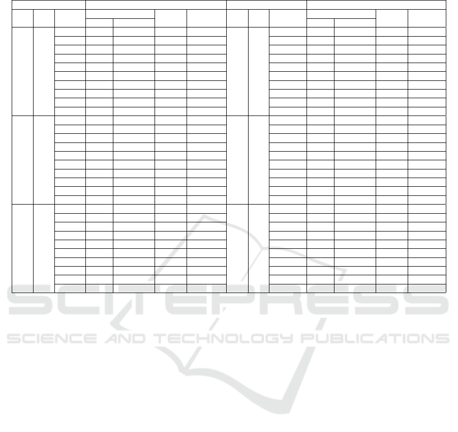
Table 2: Evaluation of MIP formulation for the LMDP-SODP with small instances (n
′
∈ {10, 20}).
Problem Instance MIP Problem Instance MIP
n
′
m Instance
Objective value
Gap (%) CPU (sec) n
′
m Instance
Objective value
Gap (%) CPU (sec)
Opt Best integer Opt Best integer
10 2
I01 233.10 — 0.00 1.46
20 2
I31 318.51 — 0.00 703.52
I02 256.81 — 0.00 3.15 I32 413.94 — 0.00 161.23
I03 205.10 — 0.00 1.31 I33 337.38 — 0.00 432.24
I04 302.12 — 0.00 3.08 I34 401.58 — 0.00 151.84
I05 245.66 — 0.00 1.82 I35 366.02 — 0.00 1126.10
I06 257.84 — 0.00 1.39 I36 426.65 — 0.00 112.20
I07 297.92 — 0.00 21.88 I37 411.28 — 0.00 172.89
I08 209.54 — 0.00 1.26 I38 332.36 — 0.00 158.10
I09 245.28 — 0.00 2.56 I39 392.38 — 0.00 147.27
I10 231.61 — 0.00 1.57 I40 365.00 — 0.00 362.51
10 3
I11 273.80 — 0.00 1.51
20 3
I41 366.27 — 0.00 2.14
I12 330.01 — 0.00 3.35 I42 359.40 — 0.00 18.27
I13 267.46 — 0.00 1.56 I43 389.16 — 0.00 215.74
I14 298.25 — 0.00 0.96 I44 376.86 — 0.00 105.12
I15 372.23 — 0.00 0.84 I45 441.09 — 0.00 769.14
I16 234.89 — 0.00 1.03 I46 336.63 — 0.00 1273.27
I17 261.39 — 0.00 1.25 I47 364.95 — 0.00 22.62
I18 349.84 — 0.00 0.90 I48 350.73 — 0.00 177.60
I19 328.50 — 0.00 1.11 I49 396.58 — 0.00 915.56
I20 324.20 — 0.00 0.81 I50 357.24 — 0.00 1808.93
10 4
I21 375.51 — 0.00 0.51
20 4
I51 404.13 — 0.00 30.65
I22 463.25 — 0.00 1.21 I52 400.03 — 0.00 12.35
I23 383.95 — 0.00 0.42 I53 412.24 — 0.00 52.80
I24 436.43 — 0.00 0.49 I54 404.74 — 0.00 46.97
I25 321.37 — 0.00 0.66 I55 359.76 — 0.00 41.21
I26 277.18 — 0.00 0.41 I56 519.44 — 0.00 157.50
I27 428.94 — 0.00 1.69 I57 354.11 — 0.00 13.51
I28 271.61 — 0.00 1.46 I58 498.71 — 0.00 47.07
I29 462.79 — 0.00 1.72 I59 382.58 — 0.00 100.31
I30 488.11 — 0.00 0.44 I60 326.83 — 0.00 150.58
The computational results presented hereafter are
structured to evaluate the effectiveness of the MIP for-
mulation across varying instance sizes. Initially, we
focus on small instances, followed by an analysis of
the model’s performance on medium-sized and large
instances.
4.3 Evaluation of MIP for
LMDP-SODP
This section presents the computational results for
the benchmark instances of the LMDP-SODP, where
we evaluate the performance of the developed MIP.
The instances are defined by n
′
∈ {10, 20, 25, 30}
and m ∈ {2, 3, 4}, where n
′
represents the number
of clients and m the number of vehicles. The in-
stances can be classified into small (n
′
∈ {10, 20}) and
medium/large (n
′
∈ {25, 30}) sets. For each value of
the combination (n
′
, m), 10 instances are generated,
resulting in a total of 120 instances.
The results are comprehensively described and de-
tailed in Table 2 for small instances and Table 3 for
medium and large instances. The analysis of the re-
sults reveals several insights:
• For small instances (n
′
∈ {10, 20}) and (m ∈
{2, 3, 4}), the MIP consistently achieves optimal
solutions within the time limit for all instances.
This demonstrates the robustness and efficiency of
the formulation in solving less complex scenarios.
• For medium instances (n
′
= 25) with m = 2, the
MIP reaches optimality in 6 out of 10 instances,
while in the remaining cases, a feasible solution
(Best Integer) is found within the 3600-second
time limit. Although not all instances are solved
optimally, the model still provides high-quality
solutions.
• When n
′
= 25 and m = 3, the model attains opti-
mal solutions in 4 out of 10 instances. Similar to
the previous case, a feasible solution is obtained
for the remaining instances within the time con-
straint, underscoring the gradual increase in com-
plexity as m grows.
• For n
′
= 25 and m = 4, the MIP model success-
fully reaches optimality in 7 out of 10 instances.
For the remaining cases, a feasible solution (Best
Integer) is still computed within the allotted time,
confirming the model’s capacity to handle higher
complexity to some extent.
• For the larger instances where n
′
= 30 and
m ∈ {2, 3}, the MIP finds optimal solutions for
only 1 out of 10 instances. Despite the difficulty
in achieving optimality, feasible solutions are ob-
An Innovative Urban Delivery System Based on Customer-Selected Addresses and Cost-Effective Driver Rates
235

Table 3: Evaluation of MIP formulation for the LMDP-SODP with medium and large instances (n
′
∈ {25, 30}).
Problem Instance MIP Problem Instance MIP
n
′
m Instance
Objective value
Gap (%) CPU (sec) n
′
m Instance
Objective value
Gap (%) CPU (sec)
Opt Best integer Opt Best integer
25 2
I61 410.77 — 0.00 722.71
30 2
I91 473.05 11.94 3600
I62 475.63 — 0.00 1097.87 I92 393.13 — 0.00 327.95
I63 556.69 4.14 3600 I93 456.47 9.46 3600
I64 359.64 — 0.00 251.74 I94 554.65 9.91 3600
I65 390.72 5.67 3600 I95 520.57 16.96 3600
I66 379.10 1.36 3600 I96 501.70 3.50 3600
I67 373.79 — 0.00 47.40 I97 403.42 2.16 3600
I68 465.86 — 0.00 148.90 I98 375.77 5.31 3600
I69 470.58 — 0.00 191.54 I99 405.62 4.37 3600
I70 378.63 5.96 3600 I100 502.25 5.36 3600
25 3
I71 471.57 7.15 3600
30 3
I101 392.42 4.37 3600
I72 433.68 — 0.00 48.10 I102 505.97 6.78 3600
I73 442.66 — 0.00 277.05 I103 559.56 2.39 3600
I74 536.17 — 0.00 60.64 I104 473.76 3.29 3600
I75 398.18 7.45 3600 I105 495.75 10.11 3600
I76 401.56 5.03 3600 I106 568.01 5.71 3600
I77 477.24 6.44 3600 I107 625.09 8.10 3600
I78 399.39 — 0.00 40.84 I108 436.01 6.77 3600
I79 398.37 2.45 3600 I109 441.01 - 0.00 787.25
I80 388.74 6.44 3600 I110 499.56 12.41 3600
25 4
I81 482.60 — 0.00 233.42
30 4
I111 557.62 5.50 3600
I82 378.77 — 0.00 222.28 I112 463.12 2.85 3600
I83 486.58 2.51 3600 I113 546.66 11.21 3600
I84 426.21 — 0.00 1463.68 I114 521.10 — 0.00 687.66
I85 585.36 — 0.00 743.51 I115 457.46 9.57 3600
I86 390.97 — 0.00 511.96 I116 562.44 — 0.00 525.87
I87 470.73 — 0.00 544.58 I117 538.89 4.34 3600
I88 447.26 1.12 3600 I118 475.30 3.67 3600
I89 459.45 3.67 3600 I119 512.53 10.81 3600
I90 523.83 — 0.00 441.01 I120 504.36 4.48 3600
tained for the other instances within the time limit,
suggesting that these cases are considerably more
challenging.
• In the case where n
′
= 30 and m = 4, the model
solves 2 out of 10 instances to optimality, with
feasible solutions (Best Integer) provided for the
remaining instances within the 3600-second time
frame. This further highlights the increased dif-
ficulty when both n
′
and m reach their maximum
values in this benchmark.
These results indicate that while the MIP formu-
lation performs well across different problem config-
urations, there is a slight decrease in performance as
the problem size and complexity increase. Nonethe-
less, the model exhibits resilience by consistently
finding solutions, either optimal or near-optimal,
within the allotted time frame.
5 CONCLUSIONS
In this study, conducted as part of a research project
on logistics and urban mobility, we addressed the Last
Mile Delivery Problem with consideration for both
Service Options and Drivers’ Preferences (LMDP-
SODP). The objective function aimed to optimize de-
livery routes to minimize the total distance traveled
by vehicles, whether they are company employees or
crowd-shippers called upon depending on the work-
load, while taking into account their preferences. To
achieve this, we developed a novel Mixed Integer Pro-
gramming (MIP) formulation to optimally solve the
problem. To evaluate the performance of our pro-
posed mathematical formulation, we conducted ex-
tensive computational experiments using generated
benchmark instances. In terms of computational ef-
ficiency, the MIP model was capable of solving all in-
stances with up to 20 clients (i.e., 40 locations) and
4 delivery vehicles. For instances with 25 and 30
clients, using 2 to 4 vehicles, optimal or feasible so-
lutions were obtained in the best cases. Furthermore,
the use of crowd-shippers with clean modes of trans-
port, delivering to regions they are most familiar with,
can have a positive impact on cost reduction, environ-
mental sustainability, and customer satisfaction.
Potential future research directions could involve
several aspects. LMD can be improved by leveraging
Artificial Intelligence techniques, such as machine
learning algorithms, reinforcement learning, and neu-
ral networks, to enhance optimization and decision-
making processes. Using eco-friendly transport and
non-professional drivers can make deliveries more
sustainable and satisfy customers. The model can also
ICORES 2025 - 14th International Conference on Operations Research and Enterprise Systems
236

include multiple alternative addresses, each with dif-
ferent time windows and costs. Additionally, delving
into the integration of advanced optimization tech-
niques, such as heuristics or metaheuristics, could ef-
fectively handle large-scale problems. Efficient lo-
gistics systems are important for dealing with urban
challenges and meeting growing delivery demands.
ACKNOWLEDGEMENTS
We would like to acknowledge the support of the
APR&D program, the Ministry of Higher Educa-
tion, Scientific Research and Innovation of Morocco,
the National Centre for Scientific and Technical Re-
search, the Mohammed VI Polytechnic University,
and the OCP Foundation for their financing of the
MILEX research project.
REFERENCES
Al Hla, Y. A., Othman, M., and Saleh, Y. (2019). Opti-
mising an eco-friendly vehicle routing problem model
using regular and occasional drivers integrated with
driver behaviour control. Journal of Cleaner Produc-
tion, 234:984–1001.
Amaral, J. C. and Cunha, C. B. (2020). An exploratory
evaluation of urban street networks for last mile dis-
tribution. Cities, 107:102916.
Anily, S. (1996). The vehicle-routing problem with deliv-
ery and back-haul options. Naval Research Logistics
(NRL), 43(3):415–434.
Archetti, C., Savelsbergh, M., and Speranza, M. G.
(2016). The vehicle routing problem with occasional
drivers. European Journal of Operational Research,
254(2):472–480.
Benmansour, R., Darvish, M., Todosijevi
´
c, R., and Zuf-
ferey, N. (2024). Variable neighbourhood search
for parallel machine scheduling with a single load-
ing server: a truck-scheduling perspective. In Supply
Chain Forum: An International Journal, pages 1–13.
Taylor & Francis.
Cardeneo, A. (2005). Modellierung und Optimierung
des B2C-Tourenplanungsproblems mit alternativen
Lieferorten und-zeiten. KIT Scientific Publishing.
Cordeau, J.-F., Gendreau, M., Laporte, G., Potvin, J.-Y., and
Semet, F. (2002). A guide to vehicle routing heuris-
tics. Journal of the Operational Research society,
53(5):512–522.
Dragomir, A. G., Van Woensel, T., and Doerner, K. F.
(2022). The pickup and delivery problem with alter-
native locations and overlapping time windows. Com-
puters & Operations Research, 143:105758.
Eksioglu, B., Vural, A. V., and Reisman, A. (2009). The
vehicle routing problem: A taxonomic review. Com-
puters & Industrial Engineering, 57(4):1472–1483.
Golden, B. L., Raghavan, S., and Wasil, E. A. (2008).
The vehicle routing problem: latest advances and new
challenges, volume 43. Springer Science & Business
Media.
Jazemi, R., Alidadiani, E., Ahn, K., and Jang, J. (2023).
A review of literature on vehicle routing problems of
last-mile delivery in urban areas. Applied Sciences,
13(24):13015.
Kiba-Janiak, M., Marcinkowski, J., Jagoda, A., and
Skowro
´
nska, A. (2021). Sustainable last mile delivery
on e-commerce market in cities from the perspective
of various stakeholders. literature review. Sustainable
Cities and Society, 71:102984.
Laporte, G. (2009). Fifty years of vehicle routing. Trans-
portation science, 43(4):408–416.
Los, J., Spaan, M. T., and Negenborn, R. R. (2018). Fleet
management for pickup and delivery problems with
multiple locations and preferences. In Dynamics in
Logistics: Proceedings of the 6th International Con-
ference LDIC 2018, Bremen, Germany, pages 86–94.
Springer.
Macrina, G., Di Puglia Pugliese, L., Guerriero, F., and La-
gan
`
a, D. (2017). The vehicle routing problem with
occasional drivers and time windows. In Optimization
and Decision Science: Methodologies and Applica-
tions: ODS, Sorrento, Italy, September 4-7, 2017 47,
pages 577–587. Springer.
Pahwa, A. and Jaller, M. (2022). A cost-based compar-
ative analysis of different last-mile strategies for e-
commerce delivery. Transportation Research Part E:
Logistics and Transportation Review, 164:102783.
Pourmohammadreza, N. and Jokar, M. R. A. (2023). A
novel two-phase approach for optimization of the last-
mile delivery problem with service options. Sustain-
ability, 15(10):8098.
Prodhon, C. and Prins, C. (2014). A survey of recent re-
search on location-routing problems. European jour-
nal of operational research, 238(1):1–17.
Strulak-W
´
ojcikiewicz, R. and Wagner, N. (2021). Explor-
ing opportunities of using the sharing economy in sus-
tainable urban freight transport. Sustainable Cities
and Society, 68:102778.
Tilk, C., Olkis, K., and Irnich, S. (2021). The last-mile ve-
hicle routing problem with delivery options. Or Spec-
trum, 43(4):877–904.
Todosijevi
´
c, R., Hanafi, S., Uro
ˇ
sevi
´
c, D., Jarboui, B., and
Gendron, B. (2017). A general variable neighbor-
hood search for the swap-body vehicle routing prob-
lem. Computers & Operations Research, 78:468–479.
Torres, F., Gendreau, M., and Rei, W. (2022a). Crowdship-
ping: An open vrp variant with stochastic destinations.
Transportation Research Part C: Emerging Technolo-
gies, 140:103677.
Torres, F., Gendreau, M., and Rei, W. (2022b). Vehicle rout-
ing with stochastic supply of crowd vehicles and time
windows. Transportation Science, 56(3):631–653.
Toth, P. and Vigo, D. (2002). The vehicle routing problem.
SIAM.
Toth, P. and Vigo, D. (2014). Vehicle routing: problems,
methods, and applications. SIAM.
An Innovative Urban Delivery System Based on Customer-Selected Addresses and Cost-Effective Driver Rates
237

United Nations, Department of Economic and Social Af-
fairs, Population Division (2022). World Popula-
tion Prospects 2022: Summary of Results. UN
DESA/POP/2022/TR/NO. 3.
Vidal, T., Laporte, G., and Matl, P. (2020). A concise
guide to existing and emerging vehicle routing prob-
lem variants. European Journal of Operational Re-
search, 286(2):401–416.
Von Boventer, E. (1961). The relationship between trans-
portation costs and location rent in transportation
problems. Journal of Regional Science, 3(2):27–40.
Watson-Gandy, C. and Dohrn, P. (1973). Depot location
with van salesmen—a practical approach. Omega,
1(3):321–329.
Webb, M. (1968). Cost functions in the location of depots
for multiple-delivery journeys. Journal of the Opera-
tional Research Society, 19(3):311–320.
ICORES 2025 - 14th International Conference on Operations Research and Enterprise Systems
238