Hyperspectral Image Compression Using Implicit Neural Representation

and Meta-Learned Based Network

Shima Rezasoltani

and Faisal Z. Qureshi

Faculty of Science, University of Ontario Institute of Technology, Oshawa, ON L1G 0C5, Canada

Keywords:

Hyperspectral Image Compression, Implicit Neural Representations.

Abstract:

Hyperspectral images capture the electromagnetic spectrum for each pixel in a scene. These often store hun-

dreds of channels per pixel, providing signiﬁcantly more information compared to a comparably sized RGB

color image. As the cost of obtaining hyperspectral images decreases, there is a need to create effective ways

for storing, transferring, and interpreting hyperspectral data. In this paper, we develop a neural compression

method for hyperspectral images. Our methodology relies on transforming hyperspectral images into implicit

neural representations, speciﬁcally neural functions that establish a correspondence between coordinates (such

as pixel locations) and features (such as pixel spectra). Instead of explicitly saving the weights of the implicit

neural representation, we record modulations that are applied to a base network that has been “meta-learned.”

These modulations serve as a compressed coding for the hyperspectral image. We conducted an assessment

of our approach using four benchmarks—Indian Pines, Jasper Ridge, Pavia University, and Cuprite—and our

ﬁndings demonstrate that the suggested method posts signiﬁcantly faster compression times when compared

to existing schemes for hyperspectral image compression.

1 INTRODUCTION

Hyperspectral images differ from grayscale images

in that they record the electromagnetic spectrum for

each pixel rather than just storing a single value per

pixel in the case of grayscale images or three val-

ues per pixel in the case of RGB images (Goetz

et al., 1985). Consequently, every pixel in a hy-

perspectral image comprises 10s or 100s of values,

which indicate the measured reﬂectance in different

frequency bands. Hyperspectral images give more

extensive opportunities for item recognition, material

identiﬁcation, and scene analysis compared to a stan-

dard color RGB image. The costs linked to acquir-

ing high-resolution hyperspectral images, which in-

clude both spatial and spectral data, are steadily de-

clining. Consequently, hyperspectral images are ﬁnd-

ing increased use in diverse ﬁelds, such as remote

sensing, biotechnology, crop analysis, environmen-

tal monitoring, food production, medical diagnosis,

pharmaceutical industry, mining, and oil & gas ex-

ploration (Liang, 2012; Carrasco et al., 2003; Afro-

mowitz et al., 1988; Kuula et al., 2012; Schuler

https://orcid.org/0000-0002-4554-5800

https://orcid.org/0000-0002-8992-3607

et al., 2012; Padoan et al., 2008; Edelman et al.,

2012; Gowen et al., 2007; Feng and Sun, 2012; Clark

and Swayze, 1995). Hyperspectral images necessi-

tate storage space that is orders of magnitude more

than that required for a color RGB image of the same

size. Therefore, there is much interest in devising ef-

fective strategies for obtaining, storing, transmitting,

and evaluating hyperspectral images. With the under-

standing that compression plays a signiﬁcant role in

the storage and transmission of hyperspectral images,

this work studies the problem of hyperspectral image

compression.

Speciﬁcally, we develop a new approach for hy-

perspectral image compression that stores a hyper-

spectral image as modulations that are applied to

the internal representations of a base network that is

shared across hyperspectral images. This work is in-

spired by (Dupont et al., 2022) that studies data ag-

nostic nueral compression, and applies the scheme

that Dupont et al. proposed to the problem of hy-

perspectral image compression. This approach of-

fers two advantages over methods that use implicit

neural representations for hyperspectral image com-

pression: 1) since the base network is shared between

multiple hyperspectral images, the method is able to

exploit spatial and spectral structural similarities be-

Qureshi, F. Z. and Rezasoltani, S.

Hyperspectral Image Compression Using Implicit Neural Representation and Meta-Learned Based Network.

DOI: 10.5220/0013121200003905

Paper published under CC license (CC BY-NC-ND 4.0)

In Proceedings of the 14th International Conference on Pattern Recognition Applications and Methods (ICPRAM 2025), pages 23-31

ISBN: 978-989-758-730-6; ISSN: 2184-4313

tween different hyperspectral images, reducing en-

coding (or compression) times; and 2) modulations

require much less space to store than the space needed

to store the “weights” of the implicit neural. While

we still need to store the weights of the base network,

this cost is amortized between multiple hyperspectral

images. The intuition behind this approach is that the

base network captures the overarching structure that is

common among multiple hyperspectral images while

the modulations store image speciﬁc details. Com-

pared to the previous approaches for hyperspectral

image compression using implicit neural representa-

tions, this method proposed in this work achieves sav-

ings both in terms of computation and storage (Reza-

soltani and Qureshi, 2024).

The proposed method is evaluated using four stan-

dard benchmarks: Indian Pines, Jasper Ridge, Pavia

University, and Cuprite. The results show that the

method presented here achieves signiﬁcantly faster

compression times as compared to a number of ex-

isting methods at similar compression rates. Further-

more that the compression quality, as measured using

Peak Signal-to-Noise Ratio (PSNR), is comparable to

that achieved by other approaches.

The rest of the paper is organized as follows. We

discuss the related work in the next section. Section 3

describes the proposed method along with the evalua-

tion metrics. Datasets, experimental setup, and com-

pression results are discussed in Section 4. Section 5

concludes the paper with a summary.

2 RELATED WORK

There has been much work in the ﬁeld of hyper-

spectral image compression. In the interest of space,

we will restrict the following discussion to learning-

based schemes for hyperspectral image compression.

The discussion presented herein is by no means com-

plete and we refer the kind reader to (Zhang et al.,

2023; Dua et al., 2020) that list various hyperspectral

image compression methods found in the literature.

Learning based schemes rely upon model training

in order to reduce both rate and distortions. Almost

all learning based methods suffer from slow encod-

ing (or compression) speeds. Oftentimes this can-

not be avoided since encoding involves at least some

sort of model training. Within the space of learning-

based schemes, autoencoders have been employed to

compress hyperspectral images (Ball

e et al., 2016).

In its simplest form, autoencoders construct lower-

dimensional latent representations of pixel spectra.

The original pixel spectra is reconstructed from these

representations to arrive at the source hyperspectral

images. Methods proposed in as (Mentzer et al.,

2018; Minnen et al., 2018) enhance an autoregres-

sive model to enhance entropy encoding. Ball

e et al.

subsequently expand these works by using hyperpri-

ors (Ball

e et al., 2018).

Implicit neural network representations have also

been studied for data compression (Dupont et al.,

2021; Dupont et al., 2022). Davies et al., for ex-

ample, uses such representations to compress 3D

meshes (Davies et al., 2020). They show that implicit

neural representations achieve better results than dec-

imated meshes. Similarly (Str

umpler et al., 2022) and

(Chen et al., 2021) uses such representations to com-

press images and videos, respectively. Zhang et al.

also studies video compression using implicit neural

representations (Zhang et al., 2021). In our previ-

ous work, we have used implicit neural representa-

tions to compress hyperspectral images (Rezasoltani

and Qureshi, 2024). Approaches that employ implicit

neural representations for “data compression” suffer

from slow encoding times.

In their 2021 paper, (Lee et al., 2021), Lee et al.

demonstrate that meta-learning sparse and parameter-

efﬁcient initializations for implicit neural representa-

tions can signiﬁcantly reduce the number of param-

eters required to represent an image at a given re-

construction quality. Paper (Str

umpler et al., 2022)

achieves signiﬁcant performance improvements over

(Dupont et al., 2021) by meta-learning an MLP

initialization, followed by quantization and entropy

coding of the MLP weights ﬁtted to images. As

stated earlier, this work is inspired by the approach

discussed in (Dupont et al., 2022) that improves

upon implicit neural network learning as presented

in (Dupont et al., 2021) by employing meta learn-

ing. Speciﬁcally, we extends our prior work (Reza-

soltani and Qureshi, 2024) by exploiting metal learn-

ing framework. We show that it is indeed possible

to lower encoding times and reduce storage needs by

using implicit neural representations within a metal

learning setting.

3 METHOD

Consider a hyperspectral image I ∈ R

W×H×C

, where

W and H denote the width and the height of this image

and C denotes the number of channels. I(x, y) ∈ R

represents the spectrum recorded at location (x, y)

where x ∈ [1, W] and y ∈ [1,H]. In our prior work, we

demonstrate that it is possible to learn implicit neural

represenations that map pixel locations to pixel spec-

tra. Speciﬁcally, we can learn a function Φ

: (x,y) 7→

I(x,y). Here, Θ represent function parameters. The

ICPRAM 2025 - 14th International Conference on Pattern Recognition Applications and Methods

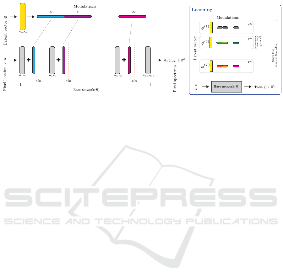
Figure 1: The base network captures the shared structure between multiple hyperspectral images; whereas, the modulations

(or latent vector) stores image-speciﬁc information. Meta learning is used to learn both the shared parameters (Θ, W

, and

) and the image speciﬁc latent vectors φ. Once an image is compressed, it is sufﬁcient to store the latent vector associated

with this image.

implicit neural network is trained by minimizing the

loss

L (I,Φ

) =

∑

∀x,y

∥I(x,y) – Φ

(x,y)∥.

Others (Tancik et al., 2020; Sitzmann et al.,

2020b) have shown that SIREN networks—multi-

layer perceptrons with Sine activation functions—

are particularly well-suited to encode high-frequency

data that sits on a grid. SIREN networks are widely

used to learn implicit neural representations. For our

purposes, a SIREN network (Φ

) comprises of K hid-

den layers. Each layer uses a sinosoidal activation

function. The K hidden features at each layer are

,··· , h

. Speciﬁcally, we deﬁne the SIREN

network as:

= sin

(

i–1

+ b

)

where h

∈ R

denotes the 2D pixel locations, W

∈

d×2

, b

∈ R

, and for i ∈ [2,K], W

∈ R

d×d

and

≂

∈ R

. The output of the network is

K+1

= W

K+1

+ b

K+1

with W

K+1

∈ R

C×d

and h

K+1

∈ R

. h

K+1

the output of the model, in our case pixel spectrum.

and b

denote the weights and biases for layer

i ∈ [1,K + 1] and represent the learnable parameters

of the network. Once this network is trained on a

given hyperspectral image, it is sufﬁcient to store the

parameters Θ = {W

|i ∈ [1, K + 1]}, since it is pos-

sible to recover the original image by evaluating Φ

at pixel locations (x, y). Savings are achieved when it

takes fewer bits to encode Φ

than those required to

encode the original image.

While we have successfully employed SIREN net-

works to compress hyperspectral images, the current

scheme suffers from two drawbacks: 1) slow com-

pression times and 2) its inability to exploit spatial

and spectral structure that is shared between hyper-

spectral images, not unlike how spatial structure is

used when analyzing RGB images. Both (1) and (2)

are due to the a fact that a new SIREN network needs

to be trained for scratch for each hyperspectral im-

age. Training is time consuming process that often re-

quires multiple epochs, and no information is shared

between multiple images.

3.1 Modulated SIREN Network

In this work we address the two shortcomings by us-

ing a meta learning approach that employs a SIREN

network (henceforth referred to as the base net-

work) that is shared between multiple hyperspec-

tral images. Image speciﬁc details are stored within

modulations—scales and shifts—applied to the fea-

tures h

, i ∈ [0,N] of the base network. This is in-

spired by the work of Perez et al., which introduced

FiLM layers (Perez et al., 2018)

FiLM(h

) = γ

⊙ h

+ β

that apply scale γ

and shift β

to a hidden feature h

Here ⊙ denotes element-wise product. Applying shift

and scale at each layer in effect allow us to parameter-

ize family of neural networks using a common (ﬁxed)

base network. Chan et al. propose a scheme where a

SIREN network is used to parameterize the generator

in a generative-adversarial setting (Chan et al., 2021).

There new samples are generated by applying modu-

lations (scale γ and shift β) as follows:

= sin



(

i–1

+ b

)

+ β



Similarly, Mehta et al. show that it is possible to pa-

rameterize a family of implicit neural representation

by applying modulations to the hidden features as

Hyperspectral Image Compression Using Implicit Neural Representation and Meta-Learned Based Network

(scale α

) (Mehta et al., 2021)

= α

⊙ sin

(

i–1

+ b

)

Both of these approach show that it is possible to map

a low-dimensional latent vector to the modulations

that are applied to the hidden features. E.g., (Chan

et al., 2021) uses an MLP to map a latent vector to

scale γ

and shift β

. Mehta et al., on the other hand,

construct the modulation α

recursively using a ﬁxed

latent vector. These schemes, however, require that

the parameters of the base network, plus the parame-

ters of the networks needed to compute the modula-

tions are stored. As a consequence these schemes are

not well-suited to the problem of data compression.

Work by Dupont et al. studied using modulations

to improve SIREN networks (Dupont et al., 2022).

They concluded that it is sufﬁcient to just use shifts

s, and that using scale modulations do not result

in a signiﬁcant improvement in performance. Fur-

thermore, their work also suggests that applying scale

modulations alone does not result in an improvement.

We follow their advice and apply shift modulations to

the features of the SIREN networks:

= sin



(

i–1

+ b

)

+ β



, (1)

here β

∈ R

. It is easy to imagine that storing

modulations β

,··· , β

takes less space than storing

weights W

and biases b

of the base network (under

the assumption that the cost of storing the base net-

work parameters is amortized over multiple images).

It is possible to achieve further savings by mapping a

low-dimensional latent vector φ ∈ R

latent

to modula-

tions. Dupont et al. also showed that it is sufﬁcient

to use a linear mapping to construct modulations β

given a latent vector, and that using a multi-layer per-

ceptron network offers little beneﬁt. Therefore, we

use a linear mapping to construct modulations given

a latent vector as:

β = W

φ + b

, (2)

with W

∈ R

(d)(K)×d

latent

and b

∈ R

(d)(K)

, the

weights and biases of the linear layer used to project

latent vector to modulations β =



|··· |β



. We re-

fer to the linear layer that maps the latent vector to

modulation as the meta network. Under this setup,

it is possible to reconstruct the original hyperspectral

image I by evaluating the modulated base network



x,y; β

,··· , β



at image pixel locations (x, y).

Similarly, when using the latent code, we can achieve

the same result by evaluating Φ



x,y; φ, Θ



, where

= {W

}, at image pixel locations (see Fig-

ure 1).

3.2 Meta Learning

Model Agnostic Meta Learning (MAML) learns an

initialization of model parameters Θ, such that, the

model can be quickly adapted to a new (related)

task (Finn et al., 2017). It has been shown that

MAML approaches can beneﬁt implicit neural repre-

sentations by reducing the number of epochs needed

to ﬁt the representation to a new data point (Sitzmann

et al., 2020a). We begin by discussing MAML within

our context. Say we are given a set of hyperspectral

images I

(1)

,··· , I

(T)

. Furthermore, assume we want

to initialize the parameters Θ of the model Φ

over

this set of images. MAML comprises of two loops:

(1) in the inner loop MAML computes image speciﬁc

update

(t)

= Θ – α

inner

∇



(t)

,Φ



;

and (2) in the outer loop it updates Θ with respect

to the performance of the model (after the inner loop

update) on the entire set:

Θ = Θ – α

outer

∇

∑

t∈[1,T]



(t)

,Φ

(t)



In practice image t is randomly chosen in the inner

loop step, and it is often sufﬁcient to sample a subset

of images in the outer loop step. The result is model

initialization parameters Θ that will allow the model

to be quickly adapted to a previously unseen hyper-

spectral image, reducing encoding in times.

The approach discussed above is not directly ap-

plicable in our setting, since we seek to learn image

speciﬁc modulations that are applied to a base net-

work that is shared between multiple hyperspectral

images. We follow the strategy discussed in (Zint-

graf et al., 2019) where they partition the parameters

into two sets. The ﬁrst set, termed context parameters,

are “task” speciﬁc and these are adapted in the inner

loop; where as, the second set is shared across “tasks”

and are meta-learned in the outer loop.

We apply this approach to our problem as fol-

lows. Given a set of hyperspectral images, parame-

ters Θ of the base networks and image speciﬁc modu-

lations β

= {β

(t)

,··· , β

(t)

}, we ﬁrst update image spe-

ciﬁc modulations in the inner loop as

(t)

= β – α

inner

∇



(t)

,Φ

[Θ|β]



;

and then update the parameters Θ in the outer loop

Θ = Θ – α

outer

∑

t∈[1,T]

∇



(t)

,Φ

[Θ|β

(t)

]



Starting value for β is ﬁxed and (Zintgraf et al., 2019)

suggests to set the initial values for β = 0. Φ

[Θ|β]

ICPRAM 2025 - 14th International Conference on Pattern Recognition Applications and Methods

denotes the modulated SIREN network (see Equa-

tion 1).

To achieve further savings, we employ linear map-

ping deﬁned in Equation 2 to construct modulations

from a given latent vector φ. As before, we can ini-

tialize φ = 0. Here, the goal is to learn image spe-

ciﬁc latent vectors φ

(t)

. The procedure is similar, ﬁrst

image speciﬁc latent vectors are updated in the inner

loop as

(t)

= φ – α

inner

∇



(t)

,Φ

[Θ

|φ]



Next, parameters Θ

are updated in the outer loop

= Θ

– α

outer

∑

t∈[1,T]

∇



(t)

,Φ

[Θ

|β

(t)

]



Here Θ

= {Θ,W

} denotes parameters of the

base network plus the parameters of the linear map-

ping used to construct modulations from latent vec-

tors. Parameters Θ

are shared between images and

latent vectors φ encode information speciﬁc to corre-

sponding image.

4 RESULTS

We selected JPEG (Good et al., 1994; Qiao et al.,

2014), JPEG2000 (Du and Fowler, 2007) and PCA-

DCT (Nian et al., 2016) schemes as baselines, since

these methods are widely deployed within the hyper-

spectral image analysis pipelines. Additionally, we

compare the method proposed with prior work that

uses implicit neural representations for hyperspectral

image compression (Rezasoltani and Qureshi, 2024).

Lastly, we will also provide compression results for

the following schemes: PCA+JPEG2000 (Du and

Fowler, 2007), FPCA+JPEG2000 (Mei et al., 2018),

RPM (Paul et al., 2016), 3D SPECK (Tang and Pearl-

man, 2006), 3D DCT (Yadav and Nagmode, 2018),

3D DWT+SVR (Zikiou et al., 2020), and WSRC

(Ouahioune et al., 2021). We employ four commonly

used hyperspectral benchmarks in this study: (1) In-

dian Pines (145×145×220); (2) Jasper Ridge (100×

100 × 224); (3) Pavia University (610 × 340 × 103);

and (4) Cuprite (614 × 512 × 224).

4.1 Metrics

Peak Signal-to-Noise Ratio (PSNR) and Mean

Squared Error (MSE) metrics are used to capture the

quality of the “compressed” image. PSNR, expressed

in decibels, is a commonly employed statistic in the

ﬁeld of image compression. It quantiﬁes the dispar-

ity in “quality” between the original image and its

compressed reproduction. A higher PSNR number in-

dicates that the compressed image closely resembles

the original image, meaning that it retains more of the

original image’s information and has superior quality.

Furthermore, we employ MSE to compare the com-

pressed image with its original version to capture the

overall differences. Smaller values of MSE indicate a

higher quality of reconstruction. MSE is computed as

follows

MSE =

∑

|I[i] –

I[i]|

, (3)

where

I denotes the compressed image and i indices

over the pixels. MSE is used to calculate PSNR

PSNR = 10 log

MSE

, (4)

where R is the largest variation in the input image in

the previous Equation.

Furthermore, the value of bits-per-pixel-per-band

(bpppb) represents the degree of compression attained

by a model. Smaller values of bpppb correspond to

greater compression rates. The bpppb of an uncom-

pressed hyperspectral image can be either 8 or 32 bits,

depending on the storage method used for the pixels.

Hyperspectral pixel values are typically stored as 32-

bit ﬂoating point numbers for each channel. The pa-

rameter bpppb is calculated as follows:

bpppb =

#parameters × (bits per parameter)

(pixels per band) × #bands

. (5)

4.2 Practical Matters

We utilize PyTorch (Paszke et al., 2019) to imple-

ment all of our models. In the inner loop, we employ

Stochastic Gradient Descent (SGD) with a learning

rate of 1e-2. In the outer loop, we utilize the Adam

optimization algorithm with a learning rate of either

1e-6 or 3e-6. Pixel locations (x,y) are converted to

normalized coordinates, i.e., (x, y) ∈ [–1, 1] × [–1,1].

Pixel spectrum values are scaled to be between 0 and

1. When the base network is shared between hyper-

spectral images having a different number of chan-

nels, we simply discard the unused channels during

loss computation.

4.3 PSNR vs. bpppb

Figure 2 plots PSNR values achieved by JPEG,

JPEG2000, PCA DCT, and INR approaches at vari-

ous bpppbs. Meta learning refers to the method de-

veloped here. The plots suggest the proposed ap-

proach achieves highest PSNR values at lower bpppb.

Hyperspectral Image Compression Using Implicit Neural Representation and Meta-Learned Based Network

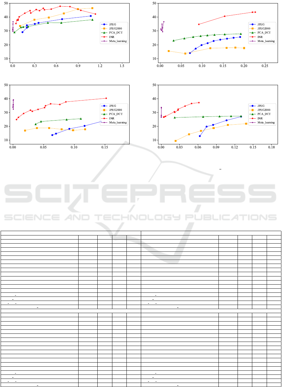
(a) Indian Pines (b) Jasper Ridge

Figure 2: PSNR vs. bpppb values. PSNR values achieved at various bpppb for our method (Meta learning), along with those

obtained by JPEG, JPEG2000, PCA-DCT, and INR schemes. x-axis represents bpppb values and y-axis represents PSNR

values.

Table 1: Compression rates on four benchmarks. For each benchmark, the ﬁrst row lists the actual size (in KB) of the original

hyperspectral image. For each method, the ﬁrst column shows the size of the compressed image (in KB), the second column

shows the PSNR achieved by comparing the decompressed image with the original image, and the third column shows the

bpppb achieved. For approaches that rely upon implicit neural representations, the structure of the network is described by

show the number of hidden layers n

and the width of these layers w

. Please note that previously K is used to denote the

number of hidden layers and d is used to denote the width of these layers, i.e. n

= K and n

= d.

Indian Pines Jasper Ridge

Method Size (KB) PSNR bpppb n

- 9251 ∞ 16 -,- - 4800 ∞ 16 -,-

JPEG (Good et al., 1994; Qiao et al., 2014) 115.6 34.085 0.2 -,- JPEG (Good et al., 1994; Qiao et al., 2014) 30 21.130 0.1 -,-

JPEG2000 (Du and Fowler, 2007) 115.6 36.098 0.2 -,- JPEG2000 (Du and Fowler, 2007) 30 17.494 0.1 -,-

PCA-DCT (Nian et al., 2016) 115.6 33.173 0.2 -,- PCA-DCT (Nian et al., 2016) 30 26.821 0.1 -,-

PCA+JPEG2000 (Du and Fowler, 2007) 115.6 39.5 0.2 -,- PCA+JPEG2000 (Du and Fowler, 2007) 30 - 0.1 -,-

FPCA+JPEG2000 (Mei et al., 2018) 115.6 40.5 0.2 -.- FPCA+JPEG2000 (Mei et al., 2018) 30 - 0.1 -,-

HEVC (Sullivan et al., 2012) 115.6 32 0.2 -,- HEVC (Sullivan et al., 2012) 30 - 0.1 -,-

RPM (Paul et al., 2016) 115.6 38 0.2 -,- RPM (Paul et al., 2016) 30 - 0.1 -,-

3D SPECK (Tang and Pearlman, 2006) 115.6 - 0.2 -,- 3D SPECK (Tang and Pearlman, 2006) 30 - 0.1 -,-

3D DCT (Yadav and Nagmode, 2018) 115.6 - 0.2 -,- 3D DCT (Yadav and Nagmode, 2018) 30 - 0.1 -,-

3D DWT+SVR (Zikiou et al., 2020) 115.6 - 0.2 -,- 3D DWT+SVR (Zikiou et al., 2020) 30 - 0.1 -,-

WSRC (Ouahioune et al., 2021) 115.6 - 0.2 -,- WSRC (Ouahioune et al., 2021) 30 - 0.1 -,-

INR (Rezasoltani and Qureshi, 2023) 115.6 40.61 0.2 15,40 INR (Rezasoltani and Qureshi, 2023) 30 35.696 0.1 10,20

HP INR (Rezasoltani and Qureshi, 2023) 57.5 40.35 0.1 15,40 HP INR (Rezasoltani and Qureshi, 2023) 15 35.467 0.06 10,20

INR sampling (Rezasoltani and Qureshi, 2024) 115.6 44.46 0.2 15,40 INR sampling (Rezasoltani and Qureshi, 2024) 30 41.58 0.1 15,20

HP INR sampling (Rezasoltani and Qureshi, 2024) 57.5 30.20 0.2 15,40 HP INR sampling (Rezasoltani and Qureshi, 2024) 15 21.48 0.06 15,20

Meta learning 2.4 36.6 0.004 5,20 Meta learning 2.3 36.6 0.008 10,60

Pavia University Cuprite

Method Size (KB) PSNR bpppb n

- 42724 ∞ 16 -,- - 140836 ∞ 16 -,-

JPEG (Good et al., 1994; Qiao et al., 2014) 267 20.253 0.1 -,- JPEG (Good et al., 1994; Qiao et al., 2014) 880.2 24.274 0.1 -,-

JPEG2000 (Du and Fowler, 2007) 267 17.752 0.1 -,- JPEG2000 (Du and Fowler, 2007) 880.2 20.889 0.1 -,-

PCA-DCT (Nian et al., 2016) 267 25.436 0.1 -,- PCA-DCT (Nian et al., 2016) 880.2 27.302 0.1 -,-

PCA+JPEG2000 (Du and Fowler, 2007) 267 - 0.1 -,- PCA+JPEG2000 (Du and Fowler, 2007) 880.2 27.5 0.1 -,-

FPCA+JPEG2000 (Mei et al., 2018) 267 - 0.1 -,- FPCA+JPEG2000 (Mei et al., 2018) 880.2 - 0.1 -,-

HEVC (Sullivan et al., 2012) 267 - 0.1 -,- HEVC (Sullivan et al., 2012) 880.2 31 0.1 -,-

RPM (Paul et al., 2016) 267 - 0.1 -,- RPM (Paul et al., 2016) 880.2 34 0.1 -,-

3D SPECK (Tang and Pearlman, 2006) 267 - 0.1 -,- 3D SPECK (Tang and Pearlman, 2006) 880.2 27.1 0.1 -,-

3D DCT (Yadav and Nagmode, 2018) 267 - 0.1 -,- 3D DCT (Yadav and Nagmode, 2018) 880.2 33.4 0.1 -,-

3D DWT+SVR (Zikiou et al., 2020) 267 - 0.1 -,- 3D DWT+SVR (Zikiou et al., 2020) 880.2 28.20 0.1 -,-

WSRC (Ouahioune et al., 2021) 267 - 0.1 -,- WSRC (Ouahioune et al., 2021) 880.2 35 0.1 -,-

INR (Rezasoltani and Qureshi, 2023) 267 33.749 0.1 20,60 INR (Rezasoltani and Qureshi, 2023) 880.2 28.954 0.1 25,100

HP INR (Rezasoltani and Qureshi, 2023) 133.5 20.886 0.05 20,60 HP INR (Rezasoltani and Qureshi, 2023) 440.1 24.334 0.06 25,100

INR sampling (Rezasoltani and Qureshi, 2024) 267 40.001 0.1 10,100 INR sampling (Rezasoltani and Qureshi, 2024) 880.2 37.007 0.1 25,100

HP INR sampling (Rezasoltani and Qureshi, 2024) 133.5 27.49 0.05 10,100 HP INR sampling (Rezasoltani and Qureshi, 2024) 440.1 24.96 0.06 25,100

Meta learning 2.1 39.1 0.0008 10,60 Meta learning 0.8 33.6 0.0001 5,60

ICPRAM 2025 - 14th International Conference on Pattern Recognition Applications and Methods

Table 2: Compression and decompression times for various methods. The proposed method (Meta learning) achieves the

fastest compression times of any method on the four benchmarks.

Dataset Method bppppb compression time (Sec) decompression time (Sec) PSNR ↑

Indian Pines

JPEG (Good et al., 1994; Qiao et al., 2014) 0.1 7.353 3.27 27.47

JPEG2000 (Du and Fowler, 2007) 0.1 0.1455 0.3115 33.58

PCA-DCT (Nian et al., 2016) 0.1 1.66 0.04 32.28

INR (Rezasoltani and Qureshi, 2023) 0.1 243.64 0 36.98

HP INR (Rezasoltani and Qureshi, 2023) 0.05 243.64 0 36.95

INR sampling (Rezasoltani and Qureshi, 2024) 0.1 132.87 0.0005 39.20

HP INR sampling (Rezasoltani and Qureshi, 2024) 0.05 132.87 0.0005 29.94

Meta learning 0.004151 0.014 0.000518 36.64

Jasper Ridge

JPEG (Good et al., 1994; Qiao et al., 2014) 0.1 3.71 1.62 24.39

JPEG2000 (Du and Fowler, 2007) 0.1 0.138 0.395 16.75

PCA-DCT (Nian et al., 2016) 0.1 1.029 0.027 25.98

INR (Rezasoltani and Qureshi, 2023) 0.1 235.19 0.0005 35.77

HP INR (Rezasoltani and Qureshi, 2023) 0.06 235.19 0.0005 35.70

INR sampling (Rezasoltani and Qureshi, 2024) 0.1 126.33 0.0005 40.20

HP INR sampling (Rezasoltani and Qureshi, 2024) 0.06 126.33 0.0005 19.58

Meta learning 0.0085 0.014 0.0004 36.67

Pavia University

JPEG (Good et al., 1994; Qiao et al., 2014) 0.1 33.86 14.61 20.86

JPEG2000 (Du and Fowler, 2007) 0.1 0.408 0.628 17.02

PCA-DCT (Nian et al., 2016) 0.1 6.525 0.235 25.121

INR (Rezasoltani and Qureshi, 2023) 0.1 352.74 0.0009 33.67

HP INR (Rezasoltani and Qureshi, 2023) 0.05 352.74 0.0009 19.75

INR sampling (Rezasoltani and Qureshi, 2024) 0.1 72.512 0.0004 38.08

HP INR sampling (Rezasoltani and Qureshi, 2024) 0.05 72.512 0.0004 27.02

Meta learning 0.0008 0.016 0.0005 39.1

Cuprite

JPEG (Good et al., 1994; Qiao et al., 2014) 0.06 101.195 45.02 12.88

JPEG2000 (Du and Fowler, 2007) 0.06 1.193 2.476 15.16

PCA-DCT (Nian et al., 2016) 0.06 11.67 0.754 26.75

INR (Rezasoltani and Qureshi, 2023) 0.06 1565.97 0.001 28.02

HP INR (Rezasoltani and Qureshi, 2023) 0.03 1565.97 0.001 27.90

INR sampling (Rezasoltani and Qureshi, 2024) 0.06 664.87 0.001 37.27

HP INR sampling (Rezasoltani and Qureshi, 2024) 0.03 664.87 0.001 24.85

Meta learning 0.0001 0.009 0.0002 33.64

Furthermore, that the proposed approach achieves

bpppb values that are less than those achieved by

other schemes.

4.4 Compression Results

Results listed in Table 1 conﬁrm that the proposed

scheme (Meta learning) achieves better PSNR and

the smallest ﬁle size (in KB) on the our bench-

marks. The table also includes compression results

achieved by other methods. Note that compression

results for every method is not available for every

benchmark; therefore, the table also contain empty

entries—for example, PSNR score for not available

for 3D SPECK scheme for Indian Pines. For every

benchmark, Meta learning achieves the highest com-

pression rate, which results in the smallest storage

requirements for the compressed image. The PSNR

scores, however, are worse than those achieved by

other methods on three of the four benchmarks: In-

dian Pines, Jasper Ridge and Cuprite. Meta learning

achieves PSNR that is similar to INR sampling on

Pavia University. Clearly, there is more work to be

done in order to improve the PSNR scores. It is worth

noting, however, that these PSNR scores are achieved

at a fraction of the storage requirements needed by

other schemes.

The key impetus of this work was to address

the slow compression times associated with implicit

neural network based hyperspectral image compres-

sion methods. Table 2 displays the compres-

sion and decompression times plus PSNR values for

various methods. The fourth column shows com-

pression times for various methods. Meta learning

achieved fastest compression times of any method on

this list. More importantly, the proposed approach

achieves compression times that are a fraction of

those posted by previous implicit neural representa-

tion based schemes.

5 CONCLUSIONS

We proposed a meta-learning approach for using im-

plicit neural representations for hyperspectral image

compression. The proposed approach shares a base

network between multiple hyperspectral images. Im-

age speciﬁc modulations store image details and these

modulations are applied to the base network to recon-

struct the original image. The results conﬁrm that the

proposed method achieves much faster compression

time when compared to existing approaches that use

implicit neural representations. We have also com-

pared our approach with a number of other schemes

for hyperspectral image compression, and the results

Hyperspectral Image Compression Using Implicit Neural Representation and Meta-Learned Based Network

conﬁrm the suitability of the method developed here

for the purposes of hyperspectral image compression.

In the future, we plan to focus on improving com-

pression quality, i.e., achieving higher PSNR scores,

while maintaining fast compression times.

REFERENCES

Afromowitz, M. A., Callis, J. B., Heimbach, D. M., DeSoto,

L. A., and Norton, M. K. (1988). Multispectral imag-

ing of burn wounds. In Medical Imaging II, volume

914, pages 500–504. SPIE.

Ball

e, J., Laparra, V., and Simoncelli, E. P. (2016). End-

to-end optimized image compression. arXiv preprint

arXiv:1611.01704.

Ball

e, J., Minnen, D., Singh, S., Hwang, S. J., and Johnston,

N. (2018). Variational image compression with a scale

hyperprior. arXiv preprint arXiv:1802.01436.

Carrasco, O., Gomez, R. B., Chainani, A., and Roper, W. E.

(2003). Hyperspectral imaging applied to medical di-

agnoses and food safety. In Geo-Spatial and Temporal

Image and Data Exploitation III, volume 5097, pages

215–221. SPIE.

Chan, E. R., Monteiro, M., Kellnhofer, P., Wu, J., and Wet-

zstein, G. (2021). pi-gan: Periodic implicit genera-

tive adversarial networks for 3d-aware image synthe-

sis. In Proceedings of the IEEE/CVF conference on

computer vision and pattern recognition, pages 5799–

5809.

Chen, H., He, B., Wang, H., Ren, Y., Lim, S. N., and Shri-

vastava, A. (2021). Nerv: Neural representations for

videos. Advances in Neural Information Processing

Systems, 34:21557–21568.

Clark, R. N. and Swayze, G. A. (1995). Mapping minerals,

amorphous materials, environmental materials, vege-

tation, water, ice and snow, and other materials: the

usgs tricorder algorithm. In JPL, Summaries of the

Fifth Annual JPL Airborne Earth Science Workshop.

Volume 1: AVIRIS Workshop.

Davies, T., Nowrouzezahrai, D., and Jacobson, A. (2020).

On the effectiveness of weight-encoded neural im-

plicit 3d shapes. arXiv preprint arXiv:2009.09808.

Du, Q. and Fowler, J. E. (2007). Hyperspectral image

compression using jpeg2000 and principal component

analysis. IEEE Geoscience and Remote sensing let-

ters, 4(2):201–205.

Dua, Y., Kumar, V., and Singh, R. S. (2020). Comprehen-

sive review of hyperspectral image compression algo-

rithms. Optical Engineering, 59(9):090902.

Dupont, E., Goli

nski, A., Alizadeh, M., Teh, Y. W.,

and Doucet, A. (2021). Coin: Compression with

implicit neural representations. arXiv preprint

arXiv:2103.03123.

Dupont, E., Loya, H., Alizadeh, M., Goli

nski, A.,

Teh, Y. W., and Doucet, A. (2022). Coin++:

Data agnostic neural compression. arXiv preprint

arXiv:2201.12904.

Edelman, G. J., Gaston, E., Van Leeuwen, T. G., Cullen,

P., and Aalders, M. C. (2012). Hyperspectral imaging

for non-contact analysis of forensic traces. Forensic

science international, 223(1-3):28–39.

Feng, Y.-Z. and Sun, D.-W. (2012). Application of hyper-

spectral imaging in food safety inspection and control:

a review. Critical reviews in food science and nutri-

tion, 52(11):1039–1058.

Finn, C., Abbeel, P., and Levine, S. (2017). Model-agnostic

meta-learning for fast adaptation of deep networks. In

International conference on machine learning, pages

1126–1135. PMLR.

Goetz, A. F., Vane, G., Solomon, J. E., and Rock, B. N.

(1985). Imaging spectrometry for earth remote sens-

ing. science, 228(4704):1147–1153.

Good, W. F., Maitz, G. S., and Gur, D. (1994). Joint pho-

tographic experts group (jpeg) compatible data com-

pression of mammograms. Journal of Digital Imag-

ing, 7(3):123–132.

Gowen, A. A., O’Donnell, C. P., Cullen, P. J., Downey, G.,

and Frias, J. M. (2007). Hyperspectral imaging–an

emerging process analytical tool for food quality and

safety control. Trends in food science & technology,

18(12):590–598.

Kuula, J., P

onen, I., Puupponen, H.-H., Selander, T.,

Reinikainen, T., Kalenius, T., and Saari, H. (2012).

Using vis/nir and ir spectral cameras for detecting and

separating crime scene details. In Sensors, and Com-

mand, Control, Communications, and Intelligence

(C3I) Technologies for Homeland Security and Home-

land Defense XI, volume 8359, page 83590P. Interna-

tional Society for Optics and Photonics.

Lee, J., Tack, J., Lee, N., and Shin, J. (2021). Meta-learning

sparse implicit neural representations. Advances in

Neural Information Processing Systems, 34:11769–

11780.

Liang, H. (2012). Advances in multispectral and hyperspec-

tral imaging for archaeology and art conservation. Ap-

plied Physics A, 106(2):309–323.

Mehta, I., Gharbi, M., Barnes, C., Shechtman, E., Ra-

mamoorthi, R., and Chandraker, M. (2021). Mod-

ulated periodic activations for generalizable local

functional representations. In Proceedings of the

IEEE/CVF International Conference on Computer Vi-

sion, pages 14214–14223.

Mei, S., Khan, B. M., Zhang, Y., and Du, Q. (2018). Low-

complexity hyperspectral image compression using

folded pca and jpeg2000. In IGARSS 2018-2018 IEEE

International Geoscience and Remote Sensing Sympo-

sium, pages 4756–4759. IEEE.

Mentzer, F., Agustsson, E., Tschannen, M., Timofte, R., and

Van Gool, L. (2018). Conditional probability mod-

els for deep image compression. In Proceedings of

the IEEE Conference on Computer Vision and Pattern

Recognition, pages 4394–4402.

Minnen, D., Ball

e, J., and Toderici, G. D. (2018). Joint

autoregressive and hierarchical priors for learned im-

age compression. Advances in neural information pro-

cessing systems, 31.

ICPRAM 2025 - 14th International Conference on Pattern Recognition Applications and Methods

Nian, Y., Liu, Y., and Ye, Z. (2016). Pairwise klt-based

compression for multispectral images. Sensing and

Imaging, 17(1):1–15.

Ouahioune, M., Ameur, S., and Lahdir, M. (2021). Enhanc-

ing hyperspectral image compression using learning-

based super-resolution technique. Earth Science In-

formatics, 14(3):1173–1183.

Padoan, R., Steemers, T., Klein, M., Aalderink, B., and

De Bruin, G. (2008). Quantitative hyperspectral imag-

ing of historical documents: technique and applica-

tions. Art Proceedings, pages 25–30.

Paszke, A., Gross, S., Massa, F., Lerer, A., Bradbury, J.,

Chanan, G., Killeen, T., Lin, Z., Gimelshein, N.,

Antiga, L., et al. (2019). Pytorch: An imperative style,

high-performance deep learning library. Advances in

neural information processing systems, 32.

Paul, M., Xiao, R., Gao, J., and Bossomaier, T.

(2016). Reﬂectance prediction modelling for residual-

based hyperspectral image coding. PloS one,

11(10):e0161212.

Perez, E., Strub, F., De Vries, H., Dumoulin, V., and

Courville, A. (2018). Film: Visual reasoning with

a general conditioning layer. In Proceedings of

the AAAI Conference on Artiﬁcial Intelligence, vol-

ume 32.

Qiao, T., Ren, J., Sun, M., Zheng, J., and Marshall, S.

(2014). Effective compression of hyperspectral im-

agery using an improved 3d dct approach for land-

cover analysis in remote-sensing applications. In-

ternational Journal of Remote Sensing, 35(20):7316–

7337.

Rezasoltani, S. and Qureshi, F. Z. (2023). Hyperspectral

image compression using implicit neural representa-

tions. In 2023 20th Conference on Robots and Vision

(CRV), pages 248–255.

Rezasoltani, S. and Qureshi, F. Z. (2024). Hyperspectral

image compression using sampling and implicit neu-

ral representations. IEEE Transactions on Geoscience

and Remote Sensing, pages 1–12.

Schuler, R. L., Kish, P. E., and Plese, C. A. (2012). Prelimi-

nary observations on the ability of hyperspectral imag-

ing to provide detection and visualization of blood-

stain patterns on black fabrics. Journal of forensic

sciences, 57(6):1562–1569.

Sitzmann, V., Chan, E., Tucker, R., Snavely, N., and Wet-

zstein, G. (2020a). Metasdf: Meta-learning signed

distance functions. Advances in Neural Information

Processing Systems, 33:10136–10147.

Sitzmann, V., Martel, J., Bergman, A., Lindell, D., and

Wetzstein, G. (2020b). Implicit neural representations

with periodic activation functions. Advances in Neu-

ral Information Processing Systems, 33:7462–7473.

Str

umpler, Y., Postels, J., Yang, R., Gool, L. V., and

Tombari, F. (2022). Implicit neural representations

for image compression. In European Conference on

Computer Vision, pages 74–91. Springer.

Sullivan, G. J., Ohm, J.-R., Han, W.-J., and Wiegand, T.

(2012). Overview of the high efﬁciency video coding

(hevc) standard. IEEE Transactions on circuits and

systems for video technology, 22(12):1649–1668.

Tancik, M., Srinivasan, P., Mildenhall, B., Fridovich-Keil,

S., Raghavan, N., Singhal, U., Ramamoorthi, R., Bar-

ron, J., and Ng, R. (2020). Fourier features let net-

works learn high frequency functions in low dimen-

sional domains. Advances in Neural Information Pro-

cessing Systems, 33:7537–7547.

Tang, X. and Pearlman, W. A. (2006). Three-dimensional

wavelet-based compression of hyperspectral images.

In Hyperspectral data compression, pages 273–308.

Springer.

Yadav, R. J. and Nagmode, M. (2018). Compression of hy-

perspectral image using pca–dct technology. In Inno-

vations in Electronics and Communication Engineer-

ing: Proceedings of the Fifth ICIECE 2016, pages

269–277. Springer.

Zhang, F., Chen, C., and Wan, Y. (2023). A survey on

hyperspectral remote sensing image compression. In

Proc. 2023 IEEE International Geoscience and Re-

mote Sensing Symposium, pages 7400–7403.

Zhang, Y., van Rozendaal, T., Brehmer, J., Nagel, M., and

Cohen, T. (2021). Implicit neural video compression.

arXiv preprint arXiv:2112.11312.

Zikiou, N., Lahdir, M., and Helbert, D. (2020). Support vec-

tor regression-based 3d-wavelet texture learning for

hyperspectral image compression. The Visual Com-

puter, 36(7):1473–1490.

Zintgraf, L., Shiarli, K., Kurin, V., Hofmann, K., and

Whiteson, S. (2019). Cavia: Fast context adapta-

tion via meta-learning. In International Conference

on Machine Learning, pages 7693–7702. PMLR.

Hyperspectral Image Compression Using Implicit Neural Representation and Meta-Learned Based Network