Deep Learning-Tuned Adaptive Inertia Weight in Particle Swarm
Optimization for Medical Image Registration
Katharina Kr
¨
amer
1 a
, Stefan M
¨
uller
1
and Michael Kosterhon
2
1
Institute of Computervisualistics, University of Koblenz, Universit
¨
atsstraße 1, 56070 Koblenz, Germany
2
Medical Center Johannes Gutenberg University, Langenbeckstraße 1, 55131 Mainz, Germany
Keywords:
Spondylodesis Surgery, Medical Image Registration, Particle Swarm Optimization, Deep Learning, Parameter
Optimization, Benchmark Functions, Search Space Volume.
Abstract:
A novel parameter training approach for Adaptive Inertia Weight Particle Swarm Optimization (AIW-PSO)
using Deep Learning is proposed. In PSO, balancing exploration and exploitation is crucial, with inertia gov-
erning parameter space sampling. This work presents a method for training transfer function parameters that
adjust the inertia weight based on a particle’s individual search ability (ISA) in each dimension. A neural net-
work is used to train the parameters of this transfer function, which then maps the ISA value to a new inertia
weight. During inference, the best possible success ratio and lowest average error are used as network inputs
to predict optimal parameters. Interestingly, the parameters across different objective functions are similar
and assume values that may appear spatially implausible, yet outperform all other considered value expres-
sions. We evaluate the proposed method Deep Learning-Tuned Adaptive Inertia Weight (TAIW) against three
inertia strategies: Constant Inertia Strategy (CIS), Linear Decreasing Inertia (LDI), Adaptive Inertia Weight
(AIW) on three benchmark functions. Additionally, we apply these PSO inertia strategies to medical image
registration, utilizing digitally reconstructed radiographs (DRRs). The results show promising improvements
in alignment accuracy using TAIW. Finally, we introduce a metric that assesses search effectiveness based on
multidimensional search space volumes.
1 INTRODUCTION
The Particle Swarm Optimization (PSO) is an es-
tablished method for solving optimization problems
across various fields. One of the central challenges in
applying PSO is achieving a balance between explo-
ration and exploitation in the search process. This bal-
ance is significantly influenced by the inertia weight,
which dominates the dynamics of particle movement.
Traditionally, different strategies for inertia have been
proposed, including constant, linearly decreasing or
even chaotic values. However, these methods do not
demonstrate optimal performance across various ap-
plications. Consequently, researchers have developed
adaptive approaches to dynamically adjust the iner-
tia weight according to the requirements of the search
process. The advancement of these adaptive strate-
gies through the incorporation of deep learning tech-
niques represents a promising step towards enhancing
PSO performance and improving efficiency. In this
a
https://orcid.org/0009-0003-1965-7512
work, we propose a novel approach based on deep
learning that dynamically adjusts the inertia param-
eters for each particle. As an outlook we propose a
metric that evaluates the success probability based on
search space volumes. Our objective is to demonstrate
the advantages of this AI-supported method through
benchmark functions and the registration of medical
images.
2 RELATED WORK
2.1 Medical Context
Medical image registration is essential in healthcare,
aligning images from various modalities like CT,
MRI, and X-ray to provide a comprehensive view of
a patient’s anatomy. This process is crucial for ap-
plications such as surgical assistance, disease diagno-
sis, and treatment planning. PSO has become a reli-
able tool for finding the appropriate transformations
Krämer, K., Müller, S. and Kosterhon, M.
Deep Learning-Tuned Adaptive Inertia Weight in Particle Swarm Optimization for Medical Image Registration.
DOI: 10.5220/0013122000003912
Paper published under CC license (CC BY-NC-ND 4.0)
In Proceedings of the 20th International Joint Conference on Computer Vision, Imaging and Computer Graphics Theory and Applications (VISIGRAPP 2025) - Volume 3: VISAPP, pages
307-318
ISBN: 978-989-758-728-3; ISSN: 2184-4321
Proceedings Copyright © 2025 by SCITEPRESS – Science and Technology Publications, Lda.
307

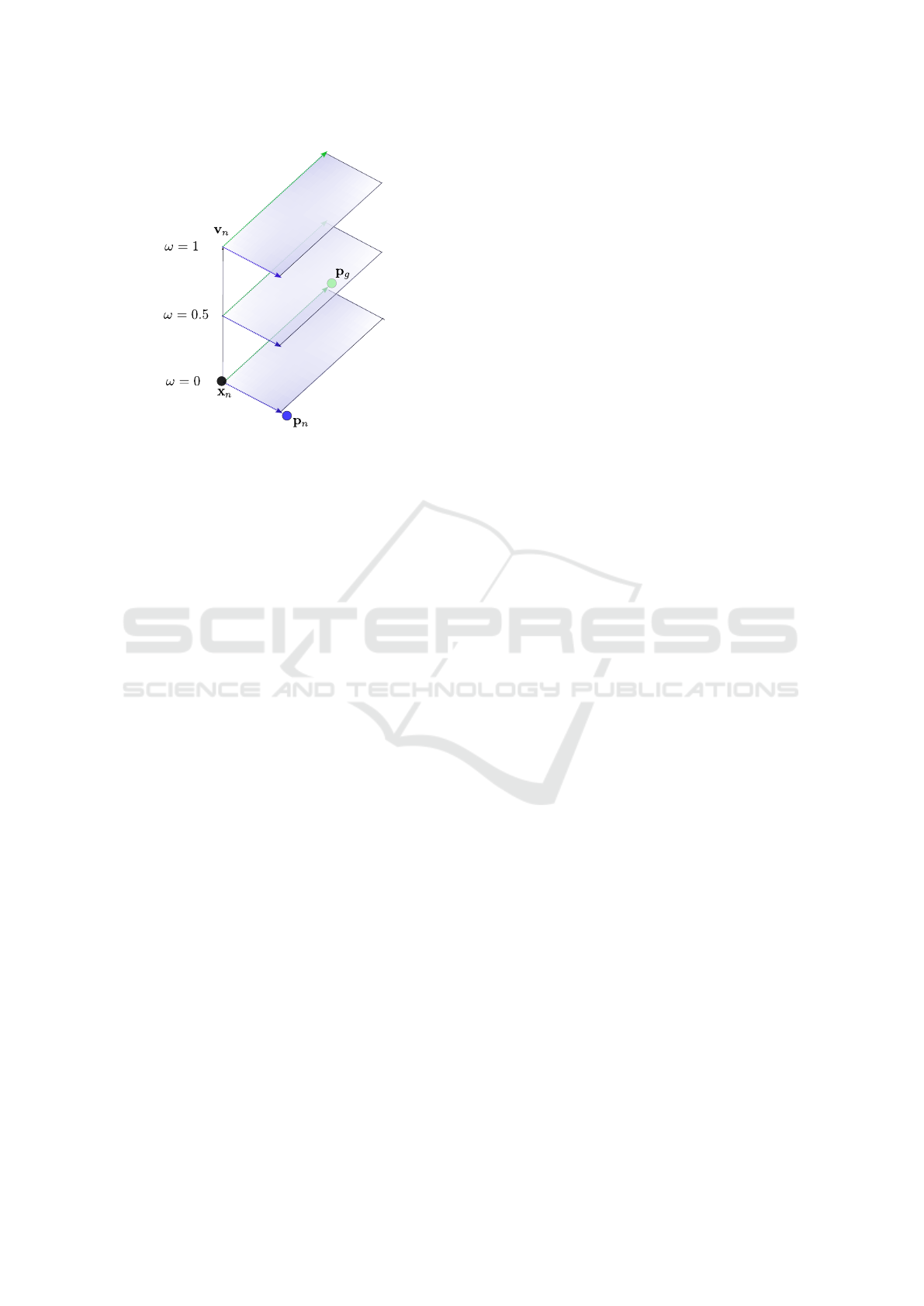
global attractor
local attractor
Figure 1: Impact of different ω values on PSO search area.
in medical image registration, effectively optimizing
multi-dimensional parameter spaces. A recent re-
view by (Ballerini, 2024) examines 24 studies utiliz-
ing PSO in this area. Two papers focus on the registra-
tion of a computed tomography volume (CT) with two
X-ray images. (Zaman and Ko, 2018) showed that
PSO is better suited for this problem than gradient-
based methods, such as Momentum Stochastic Gradi-
ent Descent (MSGD) or Nesterov Accelerated Gradi-
ent (NAG), as these methods are more prone to getting
trapped in local optima. Furthermore, (Yoon et al.,
2021) developed a multi-threaded approach, enabling
real-time registration, which highlights the potential
of PSO for practical applications in the medical field.
2.2 Particle Swarm Optimization
The Particle swarm optimization, developed by
(Kennedy and Eberhart, 1995), is a swarm-based
search algorithm that optimizes an objective function
by selecting global and local attractors in each itera-
tion to locate a global optimum. Each particle is in-
fluenced both by the social behavior of the swarm and
its own personal experience. Movement v of the n-th
particle is calculated by:
v
n
← ωv
n
+ c
1
r
1
(p
n
−x
n
) +c
2
r
2
(p
g
−x
n
) (1)
Inertia weight ω controls the influence of a par-
ticle’s previous velocity v
n
on its current movement.
Local and global attractors also guide the particle: the
local one directs it from its current position x
n
to-
ward its personal best p
n
, and the global one from
x
n
toward the global best p
g
. The magnitude of
these components is scaled by randomly chosen fac-
tors r
1
∈ [0, 1] and r
2
∈ [0, 1]. The new particle posi-
tion is x
n
← x
n
+ v
n
. In the version of PSO used in
this paper, not all particles converge at one point, but
the number of iterations is fixed. The success of the
search depends on the parameterization of ω, c
1
, and
c
2
. Typically, c
1
= c
2
is set in a range of [1.5, 2] as
in e.g. (Lu et al., 2023), (Kessentini and Barchiesi,
2015) or (Shi and Eberhart, 1998). This is done to
balance the cognitive component effecting a global
sampling (exploration) and the social component that
drives convergence (exploitation). Within our work c
1
decreases linearly from 1.5 to 0 and c
2
increases from
0 to 1.5, reflecting the need for stronger exploration
at the start and greater exploitation towards the end of
the search. Focusing only on the social and cognitive
components would oversimplify the complexities of
the optimization problem.
The inertia parameter ω introduces an additional
layer of control by physically mimicking the behavior
of individual particles in the swarm. ω plays a crucial
role in shaping the search behavior, as discussed by
(Wang et al., 2018), (Mirjalili et al., 2020) and (Shi
and Eberhart, 1998). A higher value encourages parti-
cles to explore more broadly. This helps avoiding pre-
mature convergence to local optima by exploring di-
verse regions of the search space. Conversely, a lower
inertia weight focuses the search around promising ar-
eas, enhancing the exploitation of known good solu-
tions.
As shown in Figure 1, different values of ω lead to
distinct search regions in worst case scenario if v
n
is
linearly independent of p
g
−x
n
and p
n
−x
n
. This il-
lustrates how varying the inertia weight can influence
the algorithm’s exploration of the solution space and
underscores the potential for adaptive inertia strate-
gies to improve PSO performance. Numerous meth-
ods have aimed to enhance search performance in
PSO. A simple approach is to keep ω constant at 1,
ensuring good exploration but often struggling with
convergence. A more advanced strategy involves ad-
justing ω over iterations; for example, (Shi and Eber-
hart, 1998) proposed a version where ω decreases lin-
early. (Bansal et al., 2011) found that among simple
strategies, those using random inertia values were par-
ticularly effective, highlighting the potential for adap-
tive methods.
AIW-PSO (Qin et al., 2006) introduced a basic
adaptive approach that dynamically adjusts ω based
on the fitness value of each particle, mapping it to
a new inertia value through a transfer function. The
mapping adjusts between exploration and exploita-
tion, where a lower fitness value encourages explo-
ration and a higher value promotes exploitation, thus
balancing the search strategy. Our method, TAIW-
PSO, enhances this by employing a neural network
for better selection of inertia values.
VISAPP 2025 - 20th International Conference on Computer Vision Theory and Applications
308

Additionally, (Kessentini and Barchiesi, 2015)
proposed increasing ω when particles become too
close, promoting exploration while controlling con-
vergence. Non-parametric PSO (Beheshti and Sham-
suddin, 2015) takes a different approach by dynam-
ically adjusting particle neighborhoods, initially lim-
iting influence to local neighbors and gradually ex-
panding to include all particles by the end of the
search. PSO is frequently used to optimize neural net-
works, particularly for backpropagation, as shown in
(Zhou et al., 2024). Conversely, the use of deep learn-
ing to enhance PSO parameters such as the inertia
weight ω is less common and has emerged only in re-
cent years. Several approaches have adjusted PSO pa-
rameters using Reinforcement Learning (RL). For in-
stance, (Liu et al., 2019) propose an adaptive control
algorithm for PSO based on Q-learning, where a pol-
icy network allows an agent to select optimal actions
to maximize long-term rewards. This method uses
a three-dimensional Q-table to assign actions based
on particle states. However, it is limited to only four
fixed states, restricting the variety of parameter con-
figurations that may not suffice for all particle scenar-
ios.
A survey by (Song et al., 2024) highlights the
increase in studies focusing on reinforcement learn-
ing, particularly Q-learning, over the past three years.
Among these, three notable papers enhance PSO:
(Gao et al., 2023) presents an opposition-based learn-
ing strategy to prioritize alternative objectives avoid-
ing premature convergence; (Li et al., 2023) intro-
duce a PSO variant with a neighborhood differential
mutation strategy and a dynamic oscillation inertial
weight; and (Yin et al., 2023) emphasizes adjusting
all parameters using a reward system based on ob-
served improvements. While this last approach avoids
fixed parameter values, the complexity of estimating
all three parameters simultaneously poses significant
challenges. Training a neural network to understand
the combined effects of multiple parameters can com-
plicate the training process and the interpretability of
the results. According to (Haarnoja et al., 2018), RL
presents several challenges, especially when manag-
ing complex state spaces. RL models are often tai-
lored to specific environments or tasks, making it dif-
ficult to generalize learned strategies to new or altered
situations. This limitation can be problematic in un-
predictable environments, as the adaptive capabilities
of these algorithms may become restricted. Addition-
ally, extensive training is often necessary for each spe-
cific application, which can be resource-intensive and
typically requires substantial data and computational
resources.
Given these challenges, we chose not to adopt an-
other RL approach, opting instead for a more funda-
mental strategy to approach the optimization problem
while still leveraging the advantages of deep learn-
ing technologies. For instance, the study by (Pawan
et al., 2022) demonstrates a different application of
deep learning in enhancing the PSO strategy, focus-
ing on directly training the inertia parameter ω based
on the particles’ search capabilities. Their method-
ology evaluates each particle’s behavior using Con-
volutional Neural Networks (CNNs) and Long Short-
Term Memory networks (LSTMs). In contrast, our
approach simplifies this process by learning the trans-
fer function proposed by (Qin et al., 2006), which
maps the individual search ability of each particle to a
new inertia value. This makes our method less depen-
dent on training data while still utilizing the strengths
of classical methods and deep learning combined.
In comparing strategies, we followed a similar ap-
proach to (Pawan et al., 2022), starting with the Con-
stant Inertia Strategy (CIS), where ω = 1, then pro-
gressing to the Linear Decreasing Inertia (LDI) strat-
egy, where ω decreases from 1 to 0 as proposed by
(Shi and Eberhart, 1998), and finally to AIW-PSO
(Qin et al., 2006), serving as the foundation for our
Deep Learning-Tuned AIW-PSO (TAIW).
3 BENCHMARK FUNCTIONS
The comparison is made with the help of three estab-
lished benchmark functions (Qin et al., 2006): Rastri-
gin function f (x), Griewank function g(x) and Rosen-
brock function h(x), where x is a n-dimensional vec-
tor.
f (x) = 10n +
n
∑
i=1

x
2
i
−10 cos(2πx
i
)

(2)
g(x) = 1 +
1
4000
n
∑
i=1
x
2
i
−
n
∏
i=1
cos

x
i
√
i

(3)
h(x) =
n−1
∑
i=1

100 ·(x
i+1
−x
2
i
)
2
+ (1 −x
i
)
2

(4)
These functions are examined in six dimensions,
as the application problem considered in Section 6
is also 6-dimensional, which makes the results more
comparable for the problem complexity of interest.
They were selected based on their differences in lo-
cal optima to examine a diverse range of scenarios.
4 INERTIA ADJUSTMENT
(Qin et al., 2006) developed a metric depicting the
individual search ability ISA
n
i
of a single particle n in
Deep Learning-Tuned Adaptive Inertia Weight in Particle Swarm Optimization for Medical Image Registration
309

0 2 4 6 8 10 12 14
0
0.2
0.4
0.6
0.8
1
ISA
n
i
ω ( )
α
= 0.4, β = 10
α = 0.3, β = 1
(Qin et al.)
α = 0.1, β = 20
ISA
n
i
n
i
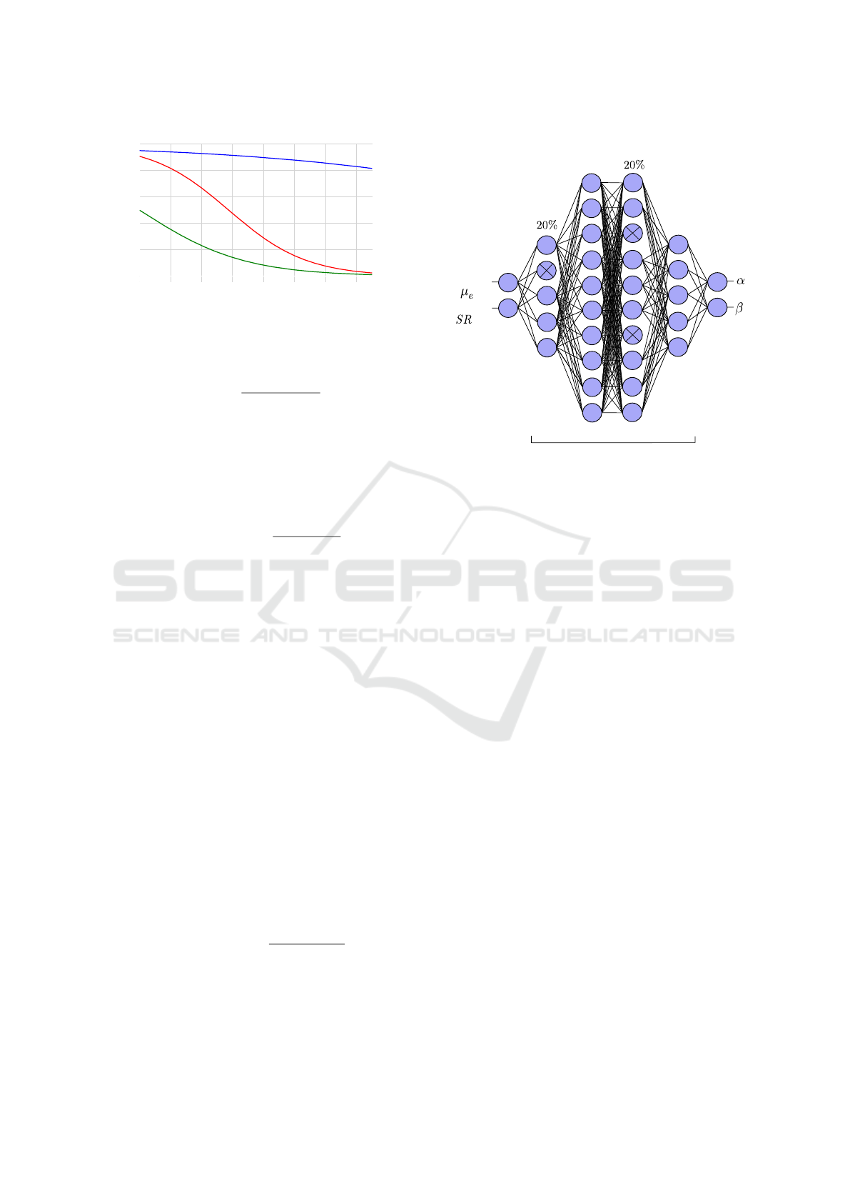
Figure 2: Possible transfer functions mapping ISA on ω.
dimension i with ε > 0:
ISA
n
i
=
|x
n
i
−p
n
i
|
|p
n
i
−p
g
i
|+ ε
(5)
A high ISA value indicates the particle is far from
its personal best and exploring new regions, while a
low ISA value suggests the particle is close to its per-
sonal best or its best is far from the global optimum.
To update ω accordingly, ISA is used in a transfer
function:
ω
n
i
(ISA
n
i
) = 1 −
1
1 + e
−αISA
n
i
(6)
We opted to adjust the formula presented in (Qin
et al., 2006) to Equation (6) due to the ambiguous
information in their paper. We had to decide be-
tween relying on the formula or the graph describ-
ing the transfer function in their work. The descrip-
tion of the impact of α on ω led us to conclude that
the graph contained the accurate information that goes
along with the authors’ intention. (Bansal et al., 2011)
show that an adaptive inertia strategy does not nec-
essarily perform better than a rudimentary approach.
Whether exploration and exploitation are successfully
balanced depends strongly on the parameterization of
the trasfer function. (Qin et al., 2006) have tested sev-
eral values for α, but using transfer function Equa-
tion (6), the inertia can never become larger than 0.5,
which has a negative impact on exploration. (Shi and
Eberhart, 1998) state that ω should be within range
[0.8, 1.2] to effectively find the global optimum. If it is
smaller than 0.8 the search is dominated by exploita-
tion and the result of the search gets more random,
converging to local minima. Therefore, we added pa-
rameter β to Equation (6):
ω
n
i
(ISA
n
i
) = 1 −
1
1 + βe
−αISA
n
i
(7)
This makes it possible to enable values of ω be-
tween 1 and 0, with different slopes, as illustrated in
Figure 2. To find the best parameters (α, β) for Equa-
tion (7) we set up a neural network that models the
dropout
random
Leaky ReLU
mean error
sucess ratio
dropout
random
Figure 3: Network architecture: fully connected layers of
shape (2-5-10-10-5-2), dropout 20%, activation function of
hidden layers: Leaky ReLU.
relationship between these parameters and the evalu-
ation metrics (µ
e
, SR) (cf. Figure 3). These metrics are
based on 100 test runs of the PSO with the respective
transfer function parameters α and β. From the re-
sults, the average error µ
e
and a success ratio SR were
calculated. A run is considered successful if the error
value falls below a threshold of 0.05. In the infer-
ence step the best possible metric-pair (0, 1) is given
as an input and the output will be the optimal param-
eters based on the training data, that is generated for
each objective function. Our approach progressively
doubling and halving the number of neurons between
layers facilitates a hierarchical feature extraction pro-
cess, enabling the network to learn and represent dif-
ferent levels of features (Bengio, 2009).
Lastly, we chose a total number of 30 hidden
neurons. Mean Squared Error was chosen as the
metric for backpropagation, Adam as the optimizer
(Kingma, 2014) and a learning rate of 0.001, as well
as 300 epochs and a batch size of 8. These param-
eters were found by trial and error, aiming to effec-
tively reduce the loss. The training dataset consists of
900 samples (α, β), with α ∈ [0.1, 0.4] and β ∈ [1, 20]
uniformly distributed, for which the PSO is run 100
times each. These runs can then be used to calcu-
late (µ
e
, SR), which then serve as the network input.
After the input layer, all values are normalized to en-
sure consistent scaling. An attempt was also made to
include the variance as a third input parameter. How-
ever, this has led to a deterioration in generalizability.
Additionally, a 20% dropout was introduced because
the validation loss was consistently higher than the
VISAPP 2025 - 20th International Conference on Computer Vision Theory and Applications
310

Table 1: Comparison of Error Variance: Mean vs. Weighted Mean Across Different Iteration Counts; Iter. = Iterations.
Iter. PSO test runs σ
2
µ
e
100 439.1 260.1 10038.4 761.4 948 221.5 474 657.5 259.9 274 9,200,804
500 329.2 449.2 2,460.4 290.8 521.5 452.6 528.3 466.5 356.3 429.7 420,430
µ
e
100 44 40.99 16.68 69.32 74.96 30.13 64.85 65.06 33.83 54.42 371
500 41.87 49.38 52.78 47.79 51.58 51.45 54.85 56.13 45.94 47.79 18.4
SR
100 0.55 0.49 0.66 0.53 0.56 0.66 0.49 0.5 0.68 0.54 0.0054
500 0.58 0.56 0.554 0.592 0.52 0.55 0.578 0.556 0.56 0.55 0.0004
training loss, which indicates overfitting.
The issue with the training data is that the net-
work can only be trained effectively if the parameters
consistently produce the same error values during the
PSO execution. However, µ
e
is sensitive to outliers,
which increases its variance. Training on values with
high variance would lead to arbitrary results. The so-
lution to this problem is to use the weighted mean µ
e
instead:
µ
e
=
∑
(x · f
kde
(x))
∑
f
kde
(x)
(8)
Kernel density estimation (KDE) was used to es-
timate the probability density function f
kde
of PSO
runs based on a smooth approximation to the distri-
bution of the data. For data generation 400 runs for
each objective function with one single distribution
were generated. Actually, KDE would have to be per-
formed for each parameter pair of the training data
set, but that would be very time-consuming and the
exact magnitude of f
kde
makes little difference. The
fixed probability distribution, centered around the op-
timum, focuses the network on this region, leading
to lower variance. As a result, the network concen-
trates more on the nuances between better parameters.
These parameters stand out more clearly because the
noise is minimal.
Several tests evaluating the performance of µ
e
and
µ
e
were then conducted using the Rosenbrock func-
tion (h(x)), with 10 sets of 100 runs each and parame-
ters (α = 0.1, β = 1) (cf. Table 1). From these, mean
µ
e
, weighted mean µ
e
and success ratio SR were cal-
culated based on the same runs. At first, the variance
decreases with an increasing number of iterations. For
instance, increasing the iterations from 100 to 500 re-
sulted in the variance dropping to 4.5% (µ
e
), 7.3%
(SR), and 4.9% (µ
e
). However, the number of itera-
tions used in training must match the number used in
the actual application of PSO, which cannot be arbi-
trarily high due to time constraints. When compar-
ing the mean to the weighted mean, several important
differences emerge. The mean is highly susceptible
to outliers, which can skew the results significantly,
especially in datasets containing extreme values. In
contrast, the weighted mean proves to be more stable,
as the weighting helps to reduce the influence of less
Table 2: Loss values across folds for Cascade and Regular
Training for optimizing Rastrigin function f (x); TL= Train-
ing Loss; VL= Validation Loss.
Fold
Cascade Regular
TL VL TL VL
0 2.132 1.858 2.183 1.821
1 1.663 1.204 1.96 1.51
2 1.403 3.093 1.869 2.868
3 1.503 1.453 2.06 1.743
4 1.436 1.832 1.991 2.159
Average 1.627 1.888 2.013 2.02
frequent or extreme values, providing a more accurate
representation of the data’s central tendency.
For the training process we developed a modi-
fied version of the traditional cross-validation (Berrar
et al., 2019), which can be described as a cascading
training. Instead of training multiple models and se-
lecting the best one, this approach involves contin-
uously training a single model across different data
folds. As the model sees new sections of the data pro-
gressively, it continuously improves, rather than be-
ing reset after each fold. Table 2 shows the results
of the Cascade training and regular training across
five folds. As can be seen, the Cascade approach
achieves a lower average training loss and validation
loss. These results suggest that the Cascade train-
ing strategy leads to better adaptation to the training
data and generalization indicated by the lower valida-
tion loss. This occurs because the model incremen-
tally learns from the entire dataset without being re-
set, with the training gradually adapting to the data
fold by fold. The range for the desired parameters
(α, β) was initially unclear when creating the train-
ing dataset. During the neural network’s initial train-
ing, it was found that β could take negative values,
with output parameters for the Rosenbrock function
being [0.5641866, −0.6367712]. This leads to a hy-
perbola for the transfer function, where only the pos-
itive range is relevant, as ISA ≥ 0. The hyperbola
is adjusted by the parameters so that ω falls within
[−1.747, 0), causing particles to move in the opposite
direction of their previous trajectories. To enhance re-
sults, the training data was refined to α ∈ [0.4, 1] and
β ∈ [−1, 0].
Deep Learning-Tuned Adaptive Inertia Weight in Particle Swarm Optimization for Medical Image Registration
311

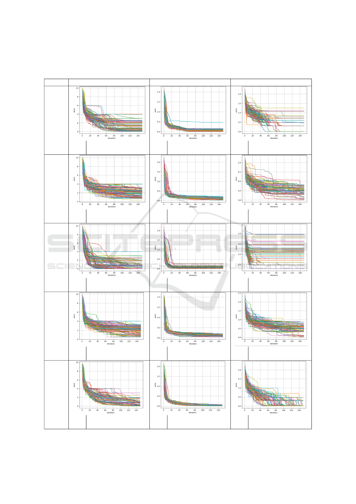
Table 3: Evaluation of benchmark functions h(x), g(x) and f (x) that are optimized by different PSO inertia strategies namely
LDI, CIS and AIW with different transfer functions that can be seen in Figure 2; evaluation metrics are mean µ
e
and success
ratio SR with tolerance threshold 0.05; Each plot depicts the iterations versus the logarithmized error for better visibility.
PSO Rosenbrock function h(x) Griewank function g(x) Rastrigin function f (x)
LDI
µ
e
703.223
SR 0.11
µ
e
0.194
SR 0.02
µ
e
2.961
SR 0.05
CIS
µ
e
963.6
SR 0
µ
e
0.288
SR 0
µ
e
2.162
SR 0.01
AIW
α= 0.3
β = 1
µ
e
394.388
SR 0.41
µ
e
0.149
SR 0.18
µ
e
9.77
SR 0
AIW
α= 0.1
β = 20
µ
e
715.671
SR 0
µ
e
0.277
SR 0
µ
e
2.178
SR 0.01
AIW
α= 0.4
β = 10
µ
e
60.64
SR 0.15
µ
e
0.068
SR 0.31
µ
e
0.363
SR 0.65
VISAPP 2025 - 20th International Conference on Computer Vision Theory and Applications
312

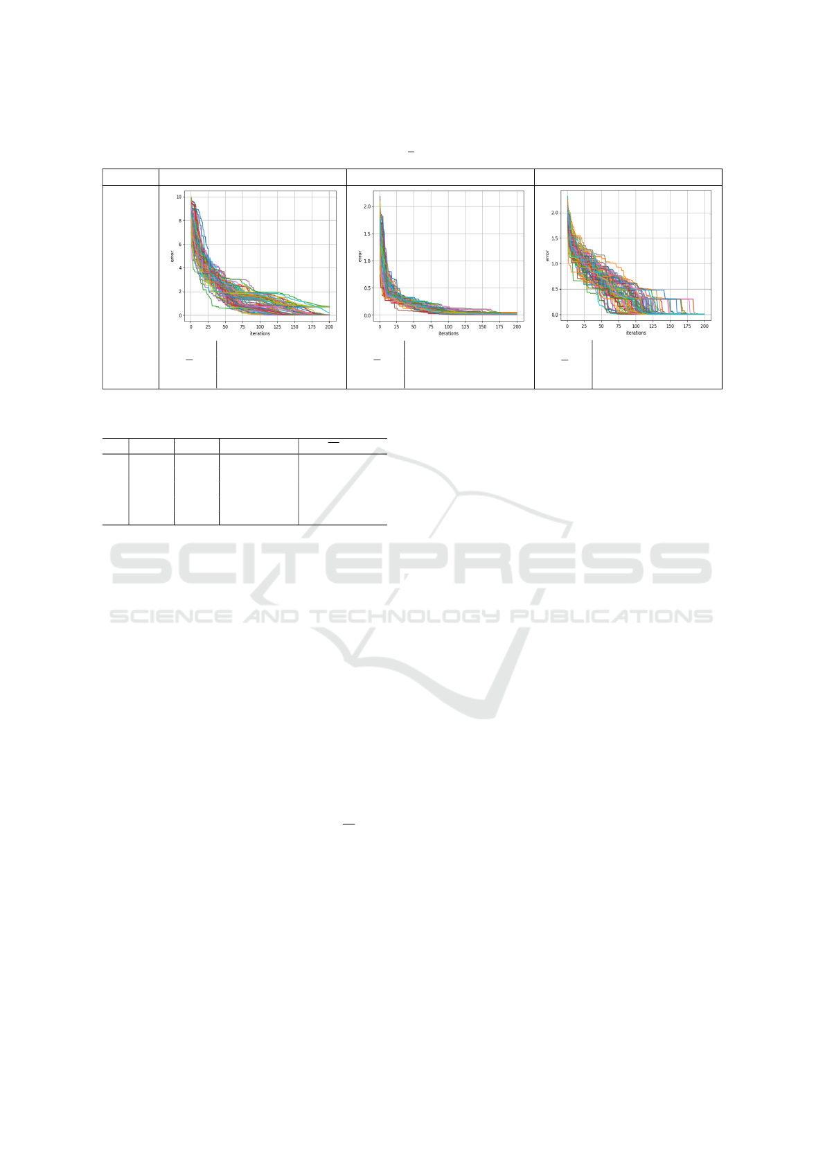
Table 4: Evaluation of benchmark functions h(x), g(x) and f (x) that are optimized by TAIW-PSO where α and β are computed
by the neural network; evaluation metrics are weighted mean µ
e
and success ratio SR with tolerance threshold 0.05.
PSO Rosenbrock function h(x) Griewank function g(x) Rastrigin function f (x)
TAIW
(α, β) (0.793, -0.793)
µ
e
0.457
SR 0.83
(α, β) (0.627, -0.864)
µ
e
0.051
SR 0.54
(α, β) (0.81, -0.975)
µ
e
12 ×10
−6
SR 1
Table 5: Mean loss and loss variance for different models m
(Rastrigin function f (x)).
m Loss σ
2
(α, β) (µ
e
, SR)
1 1.522 25.62 (0.68, -1.05) (0.24, 0.58)
2 1.604 25.76 (0.37, -0.31) (12.7, 0)
3 1.582 25.53 (0.81, -0.98) (12 ×10
−6
, 1)
4 1.551 26.45 (0.64, -0.92) (0.01, 0.89)
5 1.524 24.84 (0.76, -0.68) (0.26, 0.67)
5 EXPERIMENTS AND
EVALUATION
To evaluate model performance, we consider the
mean average loss and variance of the loss values. A
low mean loss indicates good predictions, while vari-
ance reflects the consistency of model performance.
However, these metrics did not reliably indicate
the model’s effectiveness in capturing underlying data
patterns, as they did not correlate strongly with the
quality of outputs generated by the PSO process. Our
approach focused on training multiple models and
evaluating their outputs with the PSO algorithm, em-
phasizing outcomes over loss and variance σ
2
. Ta-
ble 5 presents the evaluation of five models trained
for the Rastrigin function. Notably, the parameters
of Model 3 yield the best results with (µ
e
, SR) =
(12×10
−6
, 1) almost reaching the ideal of (0, 1), even
though it does not have the lowest loss and variance
values. This underscores that low loss and variance
values do not necessarily correlate with the best pa-
rameter outcomes. This trend is consistent across the
other benchmark functions evaluated in this study.
First, the methods CIS, LDI, and three AIW ex-
ample cases of the transfer functions (as seen in Fig-
ure 2) will be examined using the PSO to optimize
f (x), g(x) and h(x). The results are depicted in Ta-
ble 3. Each of the plotted 100 curves describes the
course of a PSO search process, that is performed by
1000 particles, showing the best logarithmized error
for each of the 140 iterations. This way it is possible
to see whether exploration and exploitation are bal-
anced. The results are evaluated by averaged error
µ and success ratio SR. If the error drops sharply in
the first iterations, this indicates strong exploitation,
as many particles converge to and scan the promising
area. In this case the search leads to a local optimum,
shown by the error plateauing. This effect can be seen
very clearly optimizing f (x) with AIW-PSO and the
parametrization of (Qin et al., 2006) with α = 0.3 and
β = 1. On the other hand, this parametrization shows
a more controlled error decay for h(x) and g(x) com-
pared to LDI and CIS which is also reflected by the
metrics. Overall, AIW-PSO with parameters α = 0.4
and β = 10 yields the best results; however, SR for
h(x) significantly decreases. This could also change
with an increase in iterations, as the curves continue
to decline until the last iteration. So we decided to set
the iteration number to 200 for generating the training
data of TAIW.
The comparison demonstrates that the strategies
have a very different impact on the optimization suc-
cess of the functions. Although the results of Ta-
ble 3 and Table 4 cannot be directly compared due
to the differing number of iterations, the trends in the
curves indicate that TAIW provides the most balanced
search for optimizing all functions, as there are few
to no outliers. Table 4 shows the results of TAIW-
PSO. Training a model instance using the training
data takes approximately 2.4 minutes on a Intel Core
i7-12700H CPU. The parameters (α, β) cause an iner-
tia range of [−3.826, 0) for the Rosenbrock function
h(x), [−6.343, 0) for the Griewank function g(x) and
[−39.32, 0) for the Rastrigin function f (x).
Deep Learning-Tuned Adaptive Inertia Weight in Particle Swarm Optimization for Medical Image Registration
313

These intervals show that the range generally in-
creases with the risk of local optima, indicating that
functions like Rastrigin, which tend to trap the al-
gorithm, require a broader negative inertia range for
enhanced exploration. Still, it is evident that the pa-
rameters of completely different loss functions are re-
markably similar, indicating that this solution can be
generalized across various problems. In summary,
the results suggest that the neural network is able to
train correlations of data structures behind the lim-
its of the training set and finally outputs parameters
for the transfer function that cause always a nega-
tive inertia for all particles. This might seem sur-
prisingly, but during the experiments we observed no-
table changes in the swarm’s behavior using negative
inertia. The particles display a reduced tendency to
get trapped in local optima. The error decreases in
small steps, indicating that while the overall conver-
gence is slower, the particles are continuously adjust-
ing their positions and re-exploring the search space.
This behavior aligns with the idea that negative inertia
reverses particle direction, promoting more extensive
exploration and allowing the swarm to escape local
minima more effectively, without compromising the
fine-grained search of promising regions.
Our work represents an initial exploration into this
area, supported by empirical evidence of the negative
inertia’s benefits. To investigate the background fur-
ther we plan to develop an optimization analysis re-
garding the search space probability of the different
inertia strategies (see section 7).
6 MEDICAL APPLICATION
In addition to evaluating the three benchmark func-
tions, we aim to investigate the application of PSO
inertia strategies in a medical context, specifically
for optimizing camera parameters in the registration
process between X-ray images and digitally recon-
structed radiographs (DRRs)(cf. Figure 4). The gen-
eration of digitally reconstructed radiographs (DRRs)
using compute shaders in OpenGL achieves a perfor-
mance of up to 940 FPS for a resolution of (256 ×
Table 6: Statistics of emitter parameters: θ, φ, γ are angles
(in radians), and radius (r), shi f tX (sX) and shi f tY (sY) are
shifts (in millimeters).
Model
Variance of Axes
θ φ r sX sY γ
TAIW 0.02 0.0009 87 12 68 0.0005
CIS 0.022 0.001 154 15 72 0.001
LDI 0.014 0.002 252 21 60 0.002
AIW 0.009 0.001 116 17 20 0.001
a)
b)
c)
Figure 4: Registered images DRR (a), X-ray (b) and their
superimposition(c) where a) is red, and b) cyan.
256) on a NVIDIA GeForce RTX 3070 graphics card.
A single iteration of the PSO algorithm with 1, 000
particles takes 1.066 seconds. Consequently, the en-
tire optimization process with 100 iterations requires
approximately 1.8 minutes. In this study, we use a
custom-built camera model designed for optimizing
this registration problem. The camera, which gen-
erates the DRRs is modeled as a virtual emitter and
positioned in spherical coordinates around the CT
scan. The parameters (θ, φ, radius, shi f tX, shi f tY, γ)
correspond to the angular orientation and positional
shifts (in millimeters) of the virtual X-ray emitter rel-
ative to the CT scan. While a detailed description of
this camera model will be provided in a future pub-
lication, these parameters allow us to optimize the
registration process within the framework of PSO,
serving as the primary search space parametrization
for this application. The parameter space exam-
ined by the PSO in this study has the following di-
mensions: θ ∈ [1.22, 1.7], φ ∈ [1.4, 1.7], radius ∈
[350, 472], shi f tX ∈ [−10, 20], shi f tY ∈ [−10, 20]
and γ ∈ [1.5, 1.7].
The metric used as an objective function is a
feature-based comparison between DRR and X-ray
and is not discussed in depth in this paper. It is impor-
tant to note that a sufficiently accurate pose is clas-
sified as having a metric value below 27. Since the
vertebrae look very similar, the registration could be
shifted by one vertebra. Therefore, different poses can
be classified as acceptable. Furthermore the number
of iterations for this application is set to 100 due to
time constraints. The network architecture remains
consistent with the description in Section 4.
Figure 5 shows the results of the inertia strate-
gies CIS, LDI, AIW (with the proposed parameters by
Table 7: Statistics of the metric values for different inertia
strategies TAIW, CIS, LDI and AIW.
Model
Metric
Mean σ
2
TAIW 26.802 1.042
CIS 27.660 1.165
LDI 28.056 1.806
AIW 28.896 1.053
VISAPP 2025 - 20th International Conference on Computer Vision Theory and Applications
314

1.3
1.4
1.5
1.6
1.45
1.5
1.55
1.6
1.65
360
380
400
420
440
460
0
5
10
15
0
5
10
15
1.55
1.6
1.65
θ
φ
radius shiftX
shiftY
γ
1.7 1.7
26
27
28
29
30
31
1.22 1.4
472
350
20
−55
−10
20
−55
−10
1.7
1.5
pose
metric
emitter pose dimensions
1.3
1.4
1.5
1.6
θ
1.7
1.22
1.45
1.5
1.55
1.6
1.65
φ
1.7
1.4
360
380
400
420
440
460
radius
472
350
0
5
10
15
shiftX
20
−5
−10
0
5
10
15
shiftY
20
−5
−10
1.55
1.6
1.65
γ
1.7
1.5
26
27
28
29
30
31
pose
metric
emitter pose dimensions
1.3
1.4
1.5
1.6
1.45
1.5
1.55
1.6
1.65
360
380
400
420
440
460
0
5
10
15
0
5
10
15
1.55
1.6
1.65
θ
1.7
1.22
φ
1.7
1.4
radius
472
350
shiftX
20
−5
−10
shiftY
20
−5
−10
γ
1.7
1.5
26
27
28
29
30
31
pose
metric
emitter pose dimensions
1.3
1.4
1.5
1.6
1.45
1.5
1.55
1.6
1.65
360
380
400
420
440
460
0
5
10
15
0
5
10
15
1.55
1.6
1.65
θ
1.7
1.22
φ
1.7
1.4
radius
472
350
shiftX
20
−5
−10
shiftY
20
−5
−10
γ
1.7
1.5
26
27
28
29
30
31
pose
metric
emitter pose dimensions
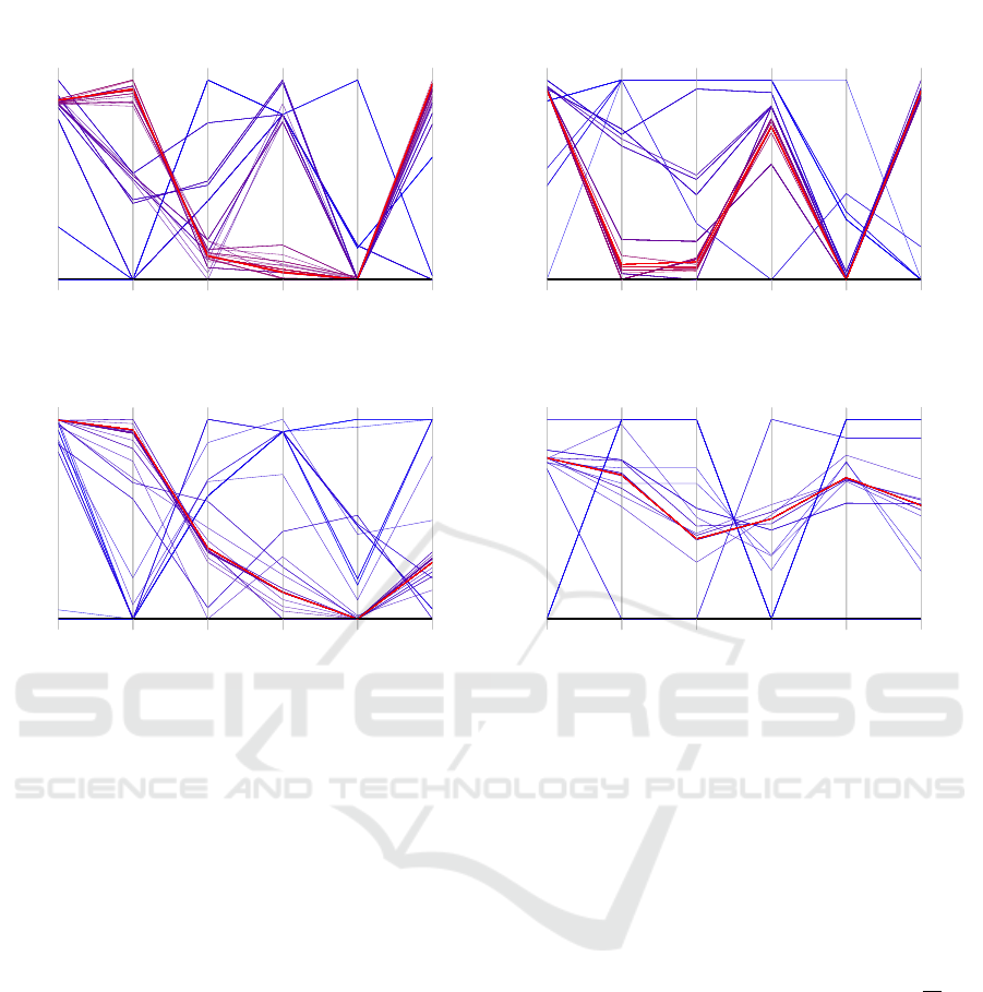
Figure 5: Visualization of the final pose results from 40 runs using the respective inertia strategy: (TAWI (upper left), CIS
(upper right), LDI (lower left), AIW (lower right)); The color coding indicates the quality of the results, with red representing
very poor outcomes and green representing very good outcomes.
(Qin et al., 2006)) and TAIW, respectively. The paral-
lel plots show six axes, one for each emitter pose di-
mension of the virtual X-ray (DRR). They are scaled
to the initial start parameter space to make the val-
ues between the PSO strategies comparable. The best
poses found by PSO in each of the 40 runs are plotted
for each strategy. The metric values range from a min-
imum of 25.38 (green) to a maximum of 31 (red). The
variances presented in Table 6 correspond to Figure 5.
These variances vary between axes due to differences
in their physical units (e.g., angles versus millime-
ter shifts). Therefore, only variances within the same
axis are directly comparable. Table 7 shows the strat-
egy specific error metric mean and metric variance
values, also corresponding to Figure 5.
TAIW not only achieves the lowest average met-
ric error value across all tested approaches, but it also
exhibits the smallest metric variance, which indicates
a high level of consistency in performance. The color
coding of the result quality based on the metric val-
ues shows that TAIW consistently produces the best
results.
Furthermore, an ANOVA (Miller Jr, 1997) was
performed to compare the performance of the four
methods, with the methods as the independent vari-
able and the metric values of all runs as the depen-
dent variable. A difference is regarded as significant
if p < 0.05. The results revealed a significant differ-
ence between the methods (F = 21.67, p < 0.0001),
indicating that at least one method outperforms the
others. Further analysis using Tukey’s HSD test (Abdi
and Williams, 2010) showed that TAIW significantly
outperforms AIW, with a mean difference of 1.987
(p = 0). Additionally, TAIW also showed significant
improvements over CIS and LDI, with mean differ-
ences of 0.8579 (p = 0.0045) and 1.2545 (p = 0),
respectively. On the other hand, AIW was found
to perform worse than both CIS and LDI, with sig-
nificant mean differences of −1.1291 (p = 0.0001)
and −0.7325 (p = 0.0212), respectively. No signif-
icant difference was observed between CIS and LDI
(p = 0.3951), suggesting that these two methods per-
form similarly. These results highlight that TAIW
provides a significant performance improvement over
the other methods, particularly AIW, and reinforces
the potential advantages of the TAIW approach.
Deep Learning-Tuned Adaptive Inertia Weight in Particle Swarm Optimization for Medical Image Registration
315

0
0.2
0.4
0.6
0.8
1
normalized dimension values
emitter pose dimensions
θ
φ
radius shiftX
shiftY
γ
0
0.2
0.4
0.6
0.8
1
normalized dimension values
emitter pose dimensions
θ
φ
radius shiftX
shiftY
γ
0
0.2
0.4
0.6
0.8
1
emitter pose dimensions
normalized dimension values
θ
φ
radius shiftX
shiftY
γ
0
0.2
0.4
0.6
0.8
1
normalized dimension values
emitter pose dimensions
θ
φ
radius shiftX
shiftY
γ
Figure 6: Visualization of the solution pose development for one PSO run using the respective inertia strategy; color coding:
blue represents the first iteration, red the final iteration, with intermediate colors interpolated per iteration (TAWI (upper left),
CIS (upper right), LDI (lower left), AIW (lower right)); values are normalized over all iterations; the best run is depicted for
every inertia strategy.
The plots in Figure 6 show the iteration progres-
sion for one specific run for each strategy. For this
purpose one specific run was selected, where the met-
ric value is at its best to analyze how the searches lead
to their best results. Iteration 1 is colored in blue and
iteration 100 is colored in red. In between the itera-
tions’ colors interpolate between blue and red. The
values are normalized to better highlight the color nu-
ances of the search behavior. This allows us to ob-
serve how far the values deviate from the initial values
and whether the search within those regions is uni-
form or more focused on specific points (helping to
investigate the convergence behavior). TAIW demon-
strates a metric value of 25.42, characterized by well-
balanced convergence properties. Each dimension
shows a smooth transition from blue to red, indicating
thorough sampling across both sides of the optimum.
The CIS strategy (cf. Figure 6), where the metric
value is 26.1, shows similar exploration properties, as
the areas around the optimum are well scanned. How-
ever, the procedure lacks the fine granularity required
for targeted convergence. Therefore, the transition
from blue to red can be recognized in much broader
levels. Conversely, AIW has a metric value of 27.46
and reveals barely any transition, marked by an abrupt
jump from blue to red, which signifies inadequate ex-
ploration. LDI strategy comes with a metric value of
25.56 and the results are similar to AIW, exhibiting
strong convergence but poor exploration capabilities.
To compensate for the reduced amount of training
data for TAIW of only 100 training pairs, several ad-
justments were made. Additionally, due to time con-
straints, the number of runs used to calculate µ
e
and
SR was reduced from 100 to 40. Although this repre-
sents a smaller sample size, it was deemed sufficient
for observing consistent patterns and trends in the
model’s performance. The batch size was decreased
from 8 to 4, allowing the model to learn more granu-
larly from smaller subsets of data. Then, the number
of training epochs was increased from 300 to 3000,
ensuring the model has sufficient time to converge and
extract meaningful patterns. Finally, the number of
folds for the cascading cross-validation approach was
increased from 5 to 10. This provides a more thor-
ough evaluation and reduces variance in the validation
process, as the model is trained and validated across
a larger variety of data splits. These adjustments col-
lectively ensure that the network generalizes well, de-
VISAPP 2025 - 20th International Conference on Computer Vision Theory and Applications
316

spite the smaller dataset. The training of the loss func-
tion used for the spondylodesis application resulted in
the parameters (α, β) = (0.72, −0.636). The inertia
value ω remains strictly negative, falling within the
range [−1.747, 0) depending on the ISA value. This
result closely resembles the values observed regard-
ing the Benchmark functions, suggesting a consistent
behavior across different loss functions and shows the
transferability to practical medical applications.
7 OUTLOOK: OPTIMIZATION
ANALYSIS
After introducing TAIW-PSO, we would like to
present an outlook on a method that provides a
stochastic interpretation of PSO. (Wang et al., 2018)
state in their outlook that there is a lack in mathe-
matical theory analysing the convergence behaviour.
Therefore, we plan to elaborate on this method in a
future paper to further investigate convergence analy-
sis of PSO examining and comparing various strate-
gies through a new perspective rather than solely re-
lying on error values. For this purpose, we aim to use
the n-ball hitting probability approach of (Chen and
Jiang, 2010), which refers to the likelihood of ran-
domly placing a particle into a n-dimensional space
and having it intersect with a specific solution space,
represented as an n-dimensional sphere. In prac-
tice, multiple solution space spheres can enclose re-
gions of interest due to the objective function’s tol-
erance, making it impractical to normalize the pa-
rameter scales to always describe the solution space
as a sphere. Instead, we define potential solution
spaces as ellipsoids, allowing the axes’ lengths to vary
freely across dimensions. The different PSO inertia
strategies result in varied probability distributions of
particle movement, leading to distinct search behav-
iors and, consequently, different success probabilities
for intersecting with these ellipsoids. Understanding
these relationships can provide insights into which
strategies are most effective for specific optimization
problems. Overmore, the probability of a particle en-
countering the solution space of the objective function
is proportional to the volume of the area enclosing all
particles, located in this solution space, in one itera-
tion step averaged over multiple runs. The core idea is
to cluster all particles from an iteration and use the in-
verse covariance matrix A to create ellipsoids, whose
volumes can then be calculated. The definition of an
ellipsoid, where x is an arbitrary point and c is the
ellipsoid center is (Gr
¨
otschel et al., 2012):
(x −c)
⊤
A(x −c) ≤ 1 (9)
Thus, this method has the potential providing a
practical approach for calculating the n-ball hitting
probability, enabling the investigation of various PSO
inertia strategies’ search behavior. This will help
broaden comparability and yield new insights into
PSO convergence analysis while reinforcing existing
findings.
8 CONCLUSION
In this paper, we developed and evaluated TAIW, an
extension of the AIW-PSO method, which integrates
deep learning to dynamically adjust the inertia weight
during the optimization process. Our approach aimed
to enhance AIW by train transfer function parame-
ters based on the individual search ability of a par-
ticle. Through extensive testing, we found that this
adaptive method, driven by learned parameters, led
to significantly better optimization results across var-
ious functions. A key aspect of our findings is the
emergence of negative inertia as a beneficial compo-
nent of the optimization process. The flexibility in-
troduced by allowing negative inertia helped prevent
the swarm from prematurely converging to local op-
tima. This resulted in more frequent re-adjustments of
the particles, allowing for a dynamic and more thor-
ough exploration of the solution space. Our exten-
sive tests demonstrated that TAIW consistently out-
performed other methods, providing the most bal-
anced and effective search strategy. In comparison
to (Pawan et al., 2022), which limits inertia weights
to positive values between 0.05 and 1, our method’s
ability to utilize negative inertia further underscores
its flexibility and effectiveness. While our training
initially started with positive inertia values, it became
clear that no positive inertia could replicate the ad-
vantages observed with negative inertia. Future work
could include a direct comparison of both methods to
explore these differences in more detail, potentially
alongside the reinforcement learning approaches.
ACKNOWLEDGEMENTS
I thank OpenAI’s ChatGPT for its help refining the
paper’s wording. The anonymized vertebra dataset
of the University of Mainz do not require ethics ap-
proval, as per Rhineland-Palatinate federal hospital
law.
Deep Learning-Tuned Adaptive Inertia Weight in Particle Swarm Optimization for Medical Image Registration
317

REFERENCES
Abdi, H. and Williams, L. J. (2010). Tukey’s honestly
significant difference (hsd) test. Encyclopedia of re-
search design, 3(1):1–5.
Ballerini, L. (2024). Particle swarm optimization in 3d med-
ical image registration: A systematic review. Archives
of Computational Methods in Engineering, pages 1–8.
Bansal, J. C., Singh, P., Saraswat, M., Verma, A., Jadon,
S. S., and Abraham, A. (2011). Inertia weight strate-
gies in particle swarm optimization. In 2011 Third
world congress on nature and biologically inspired
computing, pages 633–640. IEEE.
Beheshti, Z. and Shamsuddin, S. M. (2015). Non-
parametric particle swarm optimization for global op-
timization. Applied Soft Computing, 28:345–359.
Bengio, Y. (2009). Learning deep architectures for ai.
Berrar, D. et al. (2019). Cross-validation.
Chen, Y.-p. and Jiang, P. (2010). Analysis of particle in-
teraction in particle swarm optimization. Theoretical
Computer Science, 411(21):2101–2115.
Gao, Y.-J., Shang, Q.-X., Yang, Y.-Y., Hu, R., and Qian, B.
(2023). Improved particle swarm optimization algo-
rithm combined with reinforcement learning for solv-
ing flexible job shop scheduling problem. In Inter-
national Conference on Intelligent Computing, pages
288–298. Springer.
Gr
¨
otschel, M., Lov
´
asz, L., and Schrijver, A. (2012). Ge-
ometric algorithms and combinatorial optimization,
volume 2. Springer Science & Business Media.
Haarnoja, T., Zhou, A., Abbeel, P., and Levine, S. (2018).
Soft actor-critic: Off-policy maximum entropy deep
reinforcement learning with a stochastic actor. In
International conference on machine learning, pages
1861–1870. PMLR.
Kennedy, J. and Eberhart, R. (1995). Particle swarm opti-
mization. In Proceedings of ICNN’95-international
conference on neural networks, volume 4, pages
1942–1948. ieee.
Kessentini, S. and Barchiesi, D. (2015). Particle swarm
optimization with adaptive inertia weight. Interna-
tional Journal of Machine Learning and Computing,
5(5):368.
Kingma, D. P. (2014). Adam: A method for stochastic op-
timization. arXiv preprint arXiv:1412.6980.
Li, W., Liang, P., Sun, B., Sun, Y., and Huang, Y.
(2023). Reinforcement learning-based particle swarm
optimization with neighborhood differential mutation
strategy. Swarm and Evolutionary Computation,
78:101274.
Liu, Y., Lu, H., Cheng, S., and Shi, Y. (2019). An adaptive
online parameter control algorithm for particle swarm
optimization based on reinforcement learning. In 2019
IEEE congress on evolutionary computation (CEC),
pages 815–822. IEEE.
Lu, J., Guo, W., Liu, J., Zhao, R., Ding, Y., and Shi, S.
(2023). An intelligent advanced classification method
for tunnel-surrounding rock mass based on the parti-
cle swarm optimization least squares support vector
machine. Applied Sciences, 13(4):2068.
Miller Jr, R. G. (1997). Beyond ANOVA: basics of applied
statistics. CRC press.
Mirjalili, S., Song Dong, J., Lewis, A., and Sadiq, A. S.
(2020). Particle Swarm Optimization: Theory, Litera-
ture Review, and Application in Airfoil Design, pages
167–184. Springer International Publishing, Cham.
Pawan, Y. N., Prakash, K. B., Chowdhury, S., and Hu, Y.-
C. (2022). Particle swarm optimization performance
improvement using deep learning techniques. Multi-
media Tools and Applications, 81(19):27949–27968.
Qin, Z., Yu, F., Shi, Z., and Wang, Y. (2006). Adaptive
inertia weight particle swarm optimization. In Arti-
ficial Intelligence and Soft Computing–ICAISC 2006:
8th International Conference, Zakopane, Poland, June
25-29, 2006. Proceedings 8, pages 450–459. Springer.
Shi, Y. and Eberhart, R. (1998). A modified particle
swarm optimizer. In 1998 IEEE international confer-
ence on evolutionary computation proceedings. IEEE
world congress on computational intelligence (Cat.
No. 98TH8360), pages 69–73. IEEE.
Song, Y., Wu, Y., Guo, Y., Yan, R., Suganthan, P. N.,
Zhang, Y., Pedrycz, W., Das, S., Mallipeddi, R., Ajani,
O. S., et al. (2024). Reinforcement learning-assisted
evolutionary algorithm: A survey and research op-
portunities. Swarm and Evolutionary Computation,
86:101517.
Wang, D., Tan, D., and Liu, L. (2018). Particle swarm op-
timization algorithm: an overview. Soft computing,
22(2):387–408.
Yin, S., Jin, M., Lu, H., Gong, G., Mao, W., Chen, G., and
Li, W. (2023). Reinforcement-learning-based parame-
ter adaptation method for particle swarm optimization.
Complex & Intelligent Systems, 9(5):5585–5609.
Yoon, S., Yoon, C. H., and Lee, D. (2021). Topological
recovery for non-rigid 2d/3d registration of coronary
artery models. Computer methods and programs in
biomedicine, 200:105922.
Zaman, A. and Ko, S. Y. (2018). Improving the accuracy
of 2d-3d registration of femur bone for bone fracture
reduction robot using particle swarm optimization. In
Proceedings of the Genetic and Evolutionary Compu-
tation Conference Companion, pages 101–102.
Zhou, J., Zhao, T., Zhao, Z., and Zheng, Z. (2024). Estimat-
ing the state of charge for lithium-ion batteries in elec-
tric vehicles using the aiw-pso-bp algorithm. In 2024
4th International Conference on Electronics, Circuits
and Information Engineering (ECIE), pages 313–318.
IEEE.
VISAPP 2025 - 20th International Conference on Computer Vision Theory and Applications
318