A Ship Routing Algorithm Generating Precise and Diverse Paths

Alexandre Copp

e and Nicolas Prcovic

Aix Marseille Univ, Universit

e de Toulon, CNRS, LIS, Marseille, France

Keywords:

Sea Routing, Multicriteria Optimization, Time Dependent Algorithm.

Abstract:

We present an algorithm that accurately determines the optimal trajectories of a ship in a multi-objective and

dynamic context, where factors such as travel time and fuel consumption must be considered under varying

weather conditions during the journey. Our approach combines two recent algorithms, NAMOA*-TD and

WRM, allowing us to obtain a range of precise and diverse trajectories (a subset of the Pareto front) from which

a user can choose. Initial experiments conducted using real meteorological data demonstrate the effectiveness

of this approach.

1 INTRODUCTION

Over 80% of global trade volume is transported by

sea. In 2018, within maritime transport, 40% of op-

erational costs were absorbed by fuel expenses dur-

ing a journey. Even a small improvement, no matter

how minimal, can have signiﬁcant impacts on costs.

Therefore, routing ships based on weather conditions

is a ﬁeld of great interest for both ecological and eco-

nomic reasons.

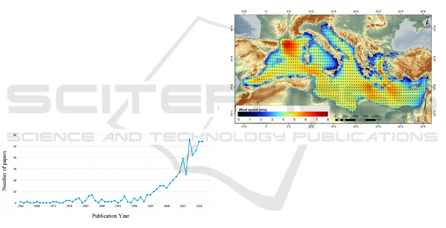
Figure 1: ”Number of publications on ship trajectories opti-

mization.” Source: Scopus February 2020.

The goal of our work is to ﬁnd a ship route be-

tween two ports, arriving before a given date, while

optimizing fuel consumption and considering envi-

ronmental constraints, all within a context that up-

dates during the journey (currents, weather). In addi-

tion to maritime geography, departure and arrival lo-

cations and dates, we must consider ocean currents

and weather conditions. These are provided in the

form of a global grid divided into rectangular cells

within which currents and wind are considered uni-

form (see ﬁg 2). This data allows us to calculate vari-

ous costs (time, fuel) associated with the route, which

depend on the wind and currents at a given moment.

Figure 2: Example of a weather grid. The arrows indicate

the direction of the wind and the colors represent its speed.

These forecasts are valid only for a speciﬁc period

(typically 6 hours), and for a journey, we need to re-

trieve the forecasts for the periods falling between the

ship’s departure and arrival dates.

Although the most realistic modeling of a ship’s

route is a continuous curve, data digitization re-

quires discretization. The digitized space and time

will therefore be a set of locations and dates, with the

number and precision of these points affecting the ef-

ﬁciency of the algorithms and the quality of the so-

lutions produced. Often, the locations are evenly dis-

tributed on a rectangular grid, forming a mesh that

covers the entire area of possible movements, aligned

with the weather grid.

The most classical approach is to represent the lo-

cations as a graph, where the edges connect vertices

corresponding to the closest locations (see Figure 3).

The edges are labeled with a cost vector (containing at

least the costs for time and fuel used to travel between

the two locations).

Tools that calculate routes in this context already

Coppé, A. and Prcovic, N.

A Ship Routing Algorithm Generating Precise and Diverse Paths.

DOI: 10.5220/0013122300003893

Paper published under CC license (CC BY-NC-ND 4.0)

In Proceedings of the 14th International Conference on Operations Research and Enterprise Systems (ICORES 2025), pages 79-87

ISBN: 978-989-758-732-0; ISSN: 2184-4372

Figure 3: Example of 8- and 16-neighbor neighborhoods

where the vertices correspond to locations evenly dis-

tributed in a rectangular grid, as used in (Chauveau, 2018).

exist and are used by maritime routing companies.

However, the solutions currently in use fall short in

at least two aspects, according to the users we spoke

with:

• The routes provided are too coarse when near the

coast.

• Often, only a single route is proposed, whereas in

a multi-objective context, there are usually a large

number of possible routes (referred to as Pareto-

optimal, see 4). However, a ship’s captain may

have preconceived notions about the best route to

take, so they may struggle to accept a single solu-

tion that differs too much from what they initially

believe to be optimal. This highlights the useful-

ness of offering a diverse set of possible solutions,

among which they are more likely to ﬁnd one that

suits them.

The structure of this article is as follows. We be-

gin by providing a formal deﬁnition of the problem

of ﬁnding an optimal route in a multi-objective and

dynamic context. Next, we present the existing algo-

rithms used to address this problem. Then, we intro-

duce our approach, based on two recent algorithms,

which allows us to obtain diverse and highly precise

routes to meet the demands of users in this ﬁeld. Fi-

nally, we present experiments based on real data pro-

vided by the maritime transport company with which

we are collaborating.

1.1 Formal Deﬁnition of the Problem

Consider a directed graph equipped with a cost func-

tion c deﬁned as: G = (N, A, c) , where N = {x

, . . . ,

} is a ﬁnite set of vertices, and A ⊂ N × N is a ﬁnite

set of |A| arcs of the form (x

). Each arc a ∈ A is

associated with a cost function vector with values in

R, of the form c(a) = (c

(a), . . . , c

(a)), where q is

the number of evaluations of the graph, and c

is the

function that assigns the i

evaluation to an arc in the

graph. s ∈ N is the source vertex of the graph (starting

point), and p ∈ N is the sink vertex of the graph (des-

tination). A solution is a path starting from the source

vertex and ending at the sink vertex.

We are interested in the optimal paths between

two vertices of the graph. Let CH

i j

be the set of paths

from x

to x

in the graph G.

We deﬁne a cost vector C which associates with

each path ch

i j

the evaluation of the costs to traverse

this path. We aim to identify the path(s) ch

i j

∈ CH

i j

such that there does not exist a path ch

′

i j

∈ CH

i j

sat-

isfying C(ch

′

i j

) < C(ch

i j

). The operator < compares

vectors, which implies a partial order on the cost of

the paths.

2 SEARCHING FOR AN

OPTIMAL PATH IN A GRAPH

There are many algorithms for searching for optimal

paths in a weighted graph, which vary depending on

whether they are single-objective or multi-objective

and whether the edge cost(s) change over time.

All these algorithms assume that the journey is

made at a constant speed. Accounting for changes

in speed or engine power during the journey intro-

duces even greater complexity, which will be consid-

ered later.

2.1 Single-Objective Algorithms

Single-objective optimization involves optimizing

only one criterion and yields a single optimal solu-

tion.

The most well-known algorithm is Dijkstra’s algo-

rithm (Dijkstra, 1959), which uses a greedy approach

to obtain an optimal solution in O(nlogn) time, where

n is the number of vertices in the graph.

The A* algorithm (Hart et al., 1968) is a variant

of Dijkstra’s algorithm, initially designed to handle

cases where the graph (too large or even inﬁnite) is

deﬁned implicitly. It evaluates a path under construc-

tion by considering not only the cost of the path al-

ready traveled (as in Dijkstra) but also a heuristic un-

derestimation of the cost of the remaining path to be

traversed.

In practice, A* allows for faster selection of the

best path and signiﬁcantly reduces the computation

time required to obtain the least costly path.

Multi-Objective Algorithms

Multi-objective algorithms aim to optimize multi-

ple criteria simultaneously, such as minimizing both

travel time and cost. These algorithms do not yield a

single optimal solution but rather a set of trade-off so-

lutions, known as Pareto-optimal solutions, where no

ICORES 2025 - 14th International Conference on Operations Research and Enterprise Systems

solution can improve one objective without worsen-

ing another.

Pareto Front. When there are multiple criteria, one

solution can only be considered better than another

if it is better on all criteria. In this case, we say that

it dominates the other solution. Some solutions, how-

ever, are incomparable: one solution may be better on

one criterion but worse on another.

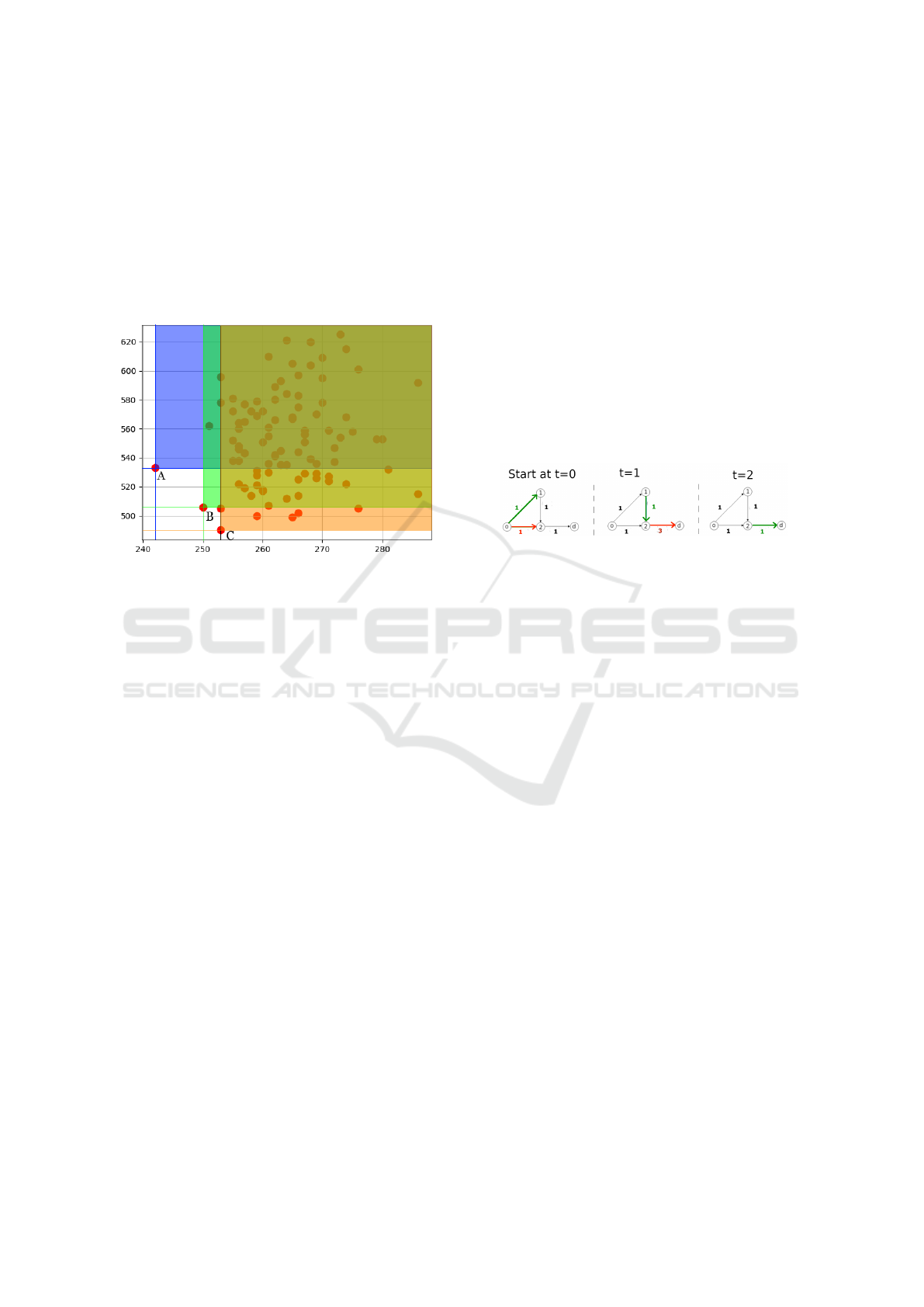
Figure 4: A solution set. In blue, green and orange are the

aeras dominated by the vertices A, B and C, which form the

Pareto front.

The set of solutions that are not dominated by any

other solution is called the Pareto front. A Pareto-

optimal solution has a cost vector such that there is

no alternative solution where any element of the cost

vector would be better.

A multi-objective problem presents the challenge

that an algorithm solving it must consider not only

the cost of the best solution to eliminate other poten-

tial candidates but all the cost vectors of the evolving

Pareto front. As a result, the problem becomes NP-

hard and potentially exhibits exponential complexity.

MOA* (Stewart and White, 1991) (Multi-

Objective A*) and NAMOA* (New Approach to

MOA*) (Mandow and De La Cruz, 2008) are general

variants of A* that take multi-objectivity into account.

Scalarization. The scalarization consists of linearly

combining different criteria to form a single one. If

we have three criteria c

, c

, and c

, the scalariza-

tion involves deﬁning the function C(c

, c

) =

+α

, where the α

are coefﬁcients to

be determined, which specify the relative importance

of each cost c

By appropriately choosing the coefﬁcients

(through dichotomic search on the parameters α

), the

entire convex hull of a Pareto front can be obtained

in polynomial time. The only solutions that will be

missing are the non-supported efﬁcient solutions.

The major advantage of scalarization is that it allows

for quick resolution; however, since it only ﬁnds the

solutions on the convex hull of the Pareto front, it is

important that this hull contains a ”good” subset of

solutions in the given context.

In the remainder of the article, we will refer to a

scalar Dijkstra as a Dijkstra algorithm that handles

multi-objective problems by scalarizing the costs.

Time-Dependent Algorithms. When the edge

costs of a graph change over time (for example, due

to weather), the property that a sub-path of an opti-

mal path is itself optimal becomes false (see Figure

5). This property can no longer be used to eliminate

suboptimal partial paths. We must use other, weaker

criteria instead.

Figure 5: On this example we have a graph at 3 different

time (0,1,2), the paradox shown is that arriving later at a

vertex with a worse cost can optimise the overall travel cost:

arriving at vertex 1 at time 2 reduces the cost (1+1+1 instead

of 1+3).

In the context of maritime routing, we can

mention the Venetti algorithm (Veneti, 2015) and

NAMOA*-TD (Chauveau, 2018). To enable the elim-

ination of candidate partial paths, these algorithms

rely on two criteria:

• The cost is higher than that of an already found

solution.

• The cost is higher than that of a partial path arriv-

ing at the same vertex at the same time.

NAMOA*-TD, a ”time-dependent” version of

NAMOA*, proves to be much more efﬁcient in prac-

tice than the Venetti algorithm (Chauveau, 2018).

This is primarily due to the fact that, unlike Venetti,

NAMOA*-TD uses a heuristic to estimate the cost of

the remaining path. This heuristic turns out to be a

sufﬁciently accurate estimate of reality, allowing it to

detect early on which candidate paths will be domi-

nated.

Although NAMOA*-TD appears to be an effec-

tive method in the context of international maritime

routing, enabling the calculation of realistic routes in

under two minutes, it has limitations that prevent it

from being fully satisfactory in our context. The rect-

angular and regular grid that determines the shape of

the trajectories is not precise enough when navigating

A Ship Routing Algorithm Generating Precise and Diverse Paths

near coasts or in narrow maritime zones (for exam-

ple, the English Channel): the maritime zone can be

narrower than the grid cells. The solution of reducing

the cell size leads to a signiﬁcant increase in compu-

tation time. For instance, halving the size of the (rect-

angular) grid cells in both dimensions quadruples the

number of vertices in the graph, in a context where the

temporal complexity of the algorithms is exponential

with respect to the number of vertices.

In practice, the tool used by the shipping company

we consulted reduces the grid sizes in certain areas

where it was found necessary afterward. The draw-

back is that the graph must be constructed somewhat

”manually,” and it is difﬁcult to precisely assess the

appropriate cell size depending on the location.

However, there is a recent approach that allows

ﬁxing the density of the trajectory of a ship with arbi-

trarily high precision, which we will be able to adapt

to our context.

2.2 The Weather Routing Metaheuristic

Approach

Weather Routing Metaheuristic (WRM) (Grandcolas,

2022) is an innovative ship routing approach that does

not predeﬁne vertices and allows for the generation of

routes where vertices can be located anywhere on the

navigable surface with an arbitrarily high degree of

precision.

The graph is determined by randomly generating

n vertices within a given area and creating an edge

between two vertices if the distance between them is

less than a speciﬁed constant. The ability to choose

n precisely allows for ﬁne-tuning the size of the in-

stance, and thus the method’s execution time. The co-

ordinates of the vertices can be determined with the

desired level of precision. The fact that vertices are

drawn randomly (uniformly) rather than placed on a

regular grid does not prevent the point density from

remaining roughly uniform across the entire naviga-

tion area.

The algorithm proceeds iteratively, ﬁrst searching

for a path in the graph and then selecting the geo-

graphic area near the vertices of the found path. It then

randomly draws n new vertices within this restricted

area to form a new graph. Gradually, the proximity

area becomes smaller, reﬁning the trajectory step by

step (see Figure 6). In WRM, an incomplete single-

objective algorithm that minimizes fuel consumption

is used, but nothing prevents the use of another single-

or multi-objective, complete or incomplete procedure.

If a multi-objective procedure is employed, multiple

paths are generated at each iteration, and only one is

selected for the next iteration.

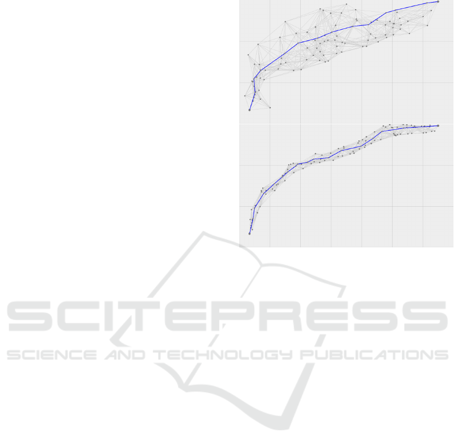
Figure 6: Step n (up) and step n + 1 (down). The geographi-

cal area of the possible locations for step n+1 is determined

by the trajectory found in step n.

3 SEARCH FOR PRECISE AND

DIVERSE ROUTES

We have seen that NAMOA*-TD allows us to obtain

a Pareto front and, therefore, all possible routes corre-

sponding to a given problem instance, but with insuf-

ﬁcient precision in a context of limited computation

time. On the other hand, WRM generates only a single

route but with a high degree of precision. To achieve

both precise and diverse routes in a short amount of

time, we propose the following simple approach:

• The ﬁrst phase of our method employs a multi-

objective algorithm in a grid (such as NAMOA*-

TD or scalar Dijkstra) to generate a Pareto front

of routes. These routes may be diverse but often

lack precision. To maximize diversity, we select a

small number (around ten among the most distant

costs) of distinct routes from the Pareto front.

• In the second phase, we reﬁne the routes gener-

ated in the ﬁrst phase using the Weather Routing

Metaheuristic (WRM). By focusing on areas sur-

rounding the initial routes, we progressively im-

prove the precision of the passage points, This

aims to gradually reﬁne a solution to reduce its

costs.

To keep the computation time short, the grid of lo-

cations used by NAMOA*-TD on a rectangular grid

ICORES 2025 - 14th International Conference on Operations Research and Enterprise Systems

must have coarser cells than if NAMOA*-TD were

used alone, allowing more time for the rest of the al-

gorithm. This results in even less precise paths than

before, but this is not an issue since they are meant to

be reﬁned immediately afterward.

For the selection of the k paths from the Pareto

front, we rely on the cost vectors and ensure that their

values are as evenly distributed as possible.

Regarding the search for Pareto-optimal paths dur-

ing an iteration of WRM, we will test two algorithms:

• NAMOA*-TD for completeness (at the cost of ex-

ecution time)

• Scalar Dijkstra, with a cost equal to a scalariza-

tion of the different costs, for speed (at the cost of

completeness).

WRM is designed to progressively narrow the area

where the vertices of the next graph may appear, fo-

cusing on the current path. However, in cases where

the current path on the new graph is not better than

the previous one, we allow ourselves to temporarily

expand this area to increase the chances of ﬁnding a

better path in the next iteration.

4 EXPERIMENTS

The current and weather data are derived from GRIB

ﬁles corresponding to real-world data. The algorithms

were tested over a 10-day weather period, with sev-

eral different routes starting at various times. We used

a 64-bit machine clocked at 2.1 GHz with 192 GB of

RAM for the experiments. So far, we have only con-

sidered two criteria: time and fuel consumption. The

fuel consumption model was provided by a shipping

company and is merely an approximation for a sin-

gle type of its vessels. All tests were conducted us-

ing the same random seed to ensure the reproducibil-

ity of results and provide a fair comparison between

different algorithm conﬁgurations. Distances are mea-

sured in degrees, and we assume that the distance of

one degree in meters is constant (ignoring the vari-

ation due to latitude). To determine the search area

around a route using WRM, we set an initial distance

d around the initial route, then multiply this distance

by 0.75 when the solution is improved and by 1.25

when there is no improvement. We limit the process

to 10 iterations. The test results presented here con-

cern a route from Boston to Lisbon on a speciﬁc date.

The other results we obtained for different dates and

between different ports do not show qualitative differ-

ences. Figure 7 shows the result of the ﬁrst part of the

algorithm, which consists of running NAMOA*-TD

on a rectangular grid.

For the second part, WRM once again uses

NAMOA*-TD. Initially, we used a scalar Dijkstra,

which was very fast but did not signiﬁcantly improve

the results.

The following ﬁgures 8, 9, and 10 show the results

of applying WRM with different initial values of d.

In the various tests, we observed that the solu-

tions tend to converge toward local minima that differ

from those found by NAMOA* during the ﬁrst phase.

Moreover, the more space we allow for divergence

around a solution, the higher the ﬁnal quality of the

solutions.

We then wanted to verify whether the initial solu-

tion quality is less important than its diversity. To do

this, in the second phase of the algorithm, we replaced

NAMOA*-TD with a scalar Dijkstra.

The results obtained are similar in quality but

much faster.

First phase NAMOA* Scalarization

(12 paths) (2 paths)

Time (s) 1610.12 7.743

Second phase NAMOA* Dijkstra Dijkstra

D = 0.5 493.284 17.892 7.112

D = 1.0 1169.74 34.475 8.647

D = 5.0 > 20 min. 565.256 127.749

5 SPEED VARIATION

So far, the approaches we have described assume

constant-speed routes. Allowing speed variation dur-

ing the journey has advantages in terms of optimizing

criteria but presents signiﬁcant drawbacks in terms of

computation time.

Allowing speed changes at each vertex of the

graph multiplies the number of choices and exponen-

tially increases computation time. However, adjusting

speed during the journey can, for example, allow a

ship to avoid certain geographic areas when weather

conditions are poor. One might plan to slow down to

pass after a storm, then speed up later to make up

for lost time. Conversely, one could speed up to pass

ahead of a storm and then slow down later to conserve

fuel for the remainder of the trip.

5.1 A Naive First Approach

We initially experimented with a naive approach that

extended our previous algorithm by allowing multi-

ple speed choices at each vertex in the graph. As ex-

pected, the computation times became too long: the

few tests conducted with ﬁve speed options resulted

in computation times of up to 1 hour and 30 min-

A Ship Routing Algorithm Generating Precise and Diverse Paths

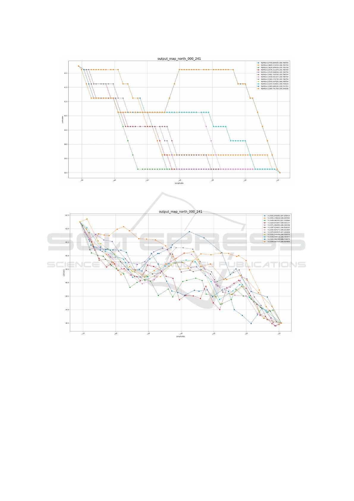
Figure 7: Set of initial solutions found by NAMOA* in a grid of 800 vertices. The pairs of values appearing in the top right

indicate, for each path, its fuel consumption and duration (in hours).

Figure 8: Improvement over 10 iterations of the initial solution with d = 0.5 and 200 vertices.

utes. Even with just three speed choices, the compu-

tation time exceeded 30 minutes. The main reason for

this inefﬁciency is that the heuristic overestimating

the remaining travel costs provides too broad bounds,

which fails to prune enough routes. Since, even when

traveling slowly at the start, one can speed up later to

make up for lost time, irrelevant paths are developed

much further compared to when speed was constant.

For this reason, we then opted for an incomplete ap-

proach.

5.2 Calculating a Single Speed via

Time/Fuel Consumption Trade-Off

To eliminate the exponential increase in computation

time caused by selecting from multiple speeds at each

vertex, we revisited the idea of scalarization, treating

the cost between two vertices as a linear combination

of time and fuel consumption. This scalarized cost de-

pends on a parameter α, which sets the relative impor-

tance of the two costs. Once α is ﬁxed, we can com-

pute a single cost between two vertices for a given

ICORES 2025 - 14th International Conference on Operations Research and Enterprise Systems

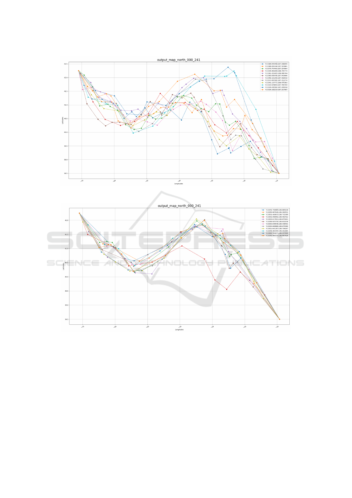
Figure 9: Improvement over 10 iterations of the initial solution with d = 1.0 and 200 vertices.

Figure 10: Improvement over 10 iterations of the initial solution with d = 5.0 and 200 vertices.

speed. The optimal speed is then chosen to minimize

this cost, knowing that this speed may vary depending

on location and time.

Our second approach, therefore, involves running

a scalar Dijkstra algorithm to determine the best route

for a ﬁxed α, calculating the optimal speed at each

new vertex. By rerunning the algorithm with different

values of α, we can offer the user a variety of route

choices.

Experimentally, the results from this approach

were somewhat disappointing. Often, the speed along

the route varies very little and remains close to an

average speed, leading to insigniﬁcant improvements

compared to maintaining a constant speed at that av-

erage. The results in terms of both computation time

and the obtained routes were quite similar to those

when the speed was kept constant.

Consequently, we ultimately decided to return to

our constant-speed route calculation algorithm but to

run it multiple times with different constant speed.

This way, we can propose additional routes to the

user, potentially diversifying the options further.

A Ship Routing Algorithm Generating Precise and Diverse Paths

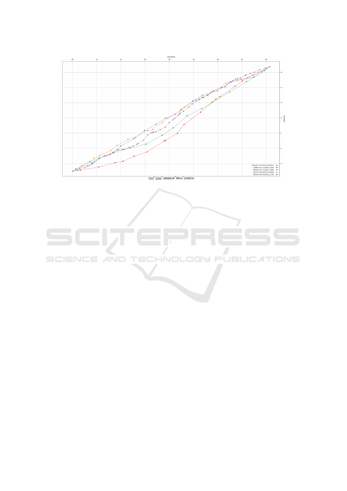
Figure 11: Multiple trajectories with constant speed.

Experimentally, choosing among several constant

speeds has, in some cases, resulted in a diversiﬁcation

of routes, as illustrated in the example shown in ﬁgure

11.

6 CONCLUSION AND FUTURE

WORK

We have proposed a method for generating diverse

and precise maritime routes in a dynamic context

where weather and ocean currents change over time.

Our approach is divided into two phases: the ﬁrst

generates diverse but imprecise and thus suboptimal

routes, followed by a second phase that reﬁnes the

passage points of the routes, improving the objectives

(time and fuel consumption).

From our initial experiments, we observed that for

both phases, a fast but incomplete algorithm (scalar

Dijkstra) was more relevant than a complete one. In-

deed, the computation times were signiﬁcantly re-

duced, while the quality of the solutions was main-

tained.

Initially, we planned to use an incomplete and

fast algorithm (scalar Dijkstra) to improve the solu-

tions generated by a complete but too slow algorithm

(NAMOA*-TD). However, we realized it was more

effective to quickly generate highly approximate so-

lutions, as the quality of these initial solutions did not

affect the quality of the ﬁnal ones.

Similarly, allowing speed variation during the

route either proved too computationally expensive or

did not lead to signiﬁcant variations when scalariz-

ing the costs. However, selecting among multiple con-

stant speeds can diversify routes in terms of the geo-

graphic areas traversed.

The results we obtained, while meeting the preci-

sion and diversiﬁcation expectations set by the ship-

ping company we collaborated with, still require fur-

ther reﬁnement. Speciﬁcally, we need a better fuel

consumption model and to incorporate additional cri-

teria (notably environmental factors). The applicabil-

ity of our approach also depends on real-world con-

straints that we still need to understand in detail: the

maximum time allocated for all calculations and the

computational resources available. These factors will

determine the ﬁnal precision of the routes our algo-

rithm can produce and, ultimately, its acceptability to

the shipping company.

ACKNOWLEDGMENTS

This work is supported by Bpifrance as part of the PIA

project ”Digital Transformation of Maritime Trans-

port” (TNTM).

REFERENCES

Chauveau, E. (2018). Optimisation des routes maritimes :

un syst

eme de r

esolution multicrit

ere et d

ependant du

temps.

Dijkstra, E. W. (1959). A note on two problems in connex-

ion with graphs. Numerische mathematik, 1(1):269–

271.

ICORES 2025 - 14th International Conference on Operations Research and Enterprise Systems

Grandcolas, S. (2022). A metaheuristic algorithm for ship

weather routing.

Hart, P. E., Nilsson, N. J., and Raphael, B. (1968). A for-

mal basis for the heuristic determination of minimum

cost paths. IEEE Transactions on Systems Science and

Cybernetics, 4(2):100–107.

Mandow, L. and De La Cruz, J. L. P. (2008). Multiob-

jective a* search with consistent heuristics. J. ACM,

Vol.57(5).

Stewart, B. S. and White, III, C. C. (1991). Multiobjective

a*. J. ACM, Vol.38(4):p.775-814.

Veneti, A., K. C. e. P. G. (2015). Continuous and discrete

time label setting algorithms for the time dependent

bi-criteria shortest path problem. Computing Society

Conference, p.62-73. 8.

A Ship Routing Algorithm Generating Precise and Diverse Paths