A Vector Autoregression Model for Depicting the Relation Between
Labour Market Economic Indicators and Real Wages in the United
States Manufacturing Sector
Ishaan Kshirsagar
1 a
, Julian M
´
arquez Simon
2 b
, Nicol
`
o Sch
¨
atz
3 c
, David Fraga Gonz
´
alez
3 d
and Conor Ryan
4,5 e
1
Department of Arts and Sciences, University College London, London, U.K.
2
Department of Economics, University College London, U.K.
3
Department of Philosophy, University College London, U.K.
4
Department of Computer Science and Information Systems, Biocomputing and Developmental Systems Research Group,
University of Limerick, Ireland
5
Lero, The Science Foundation Ireland Research Centre for Software, Ireland
Keywords:
Vector Autoregression Model, Real Wages, Time Series Analysis, US Labour Market, Manufacturing Sector.
Abstract:
In recent years, the US manufacturing sector and its labour market dynamics have gained importance in the
face of resurgent protectionism and increased governmental strategic investment plans. Simultaneously, real
wage growth in the manufacturing sector has diverged compared to the wider economy. While studies have
previously analysed the relationship between labour market conditions and real wages in the wider economy,
few have specifically evaluated the manufacturing sector in this respect. To this end, we selected a comprehen-
sive list of economic indicators covering the key aspects of the sectoral labour market. Subsequently, a vector
autoregression (VAR) model was developed, enabling us to account for time lags and the interconnectedness
of each variable. In addition to this, graphs and plots were created to provide a visual understanding of the
database, results, and labour market dynamics. The findings of our model suggest that the economic consen-
sus on real wage determination in the wider economy also holds for the manufacturing sector. An important
exception to this is the strongly negative relationship between the inflation rate and real wages.
1 INTRODUCTION
This paper examines how labour market conditions
affect changes in real wages in the United States man-
ufacturing sector between the years 2000 – 2024.
To this end, a Vector Autoregression (VAR) model
was developed using a dataset compiled from vari-
ous U.S. government databases (Federal Reserve Eco-
nomic Data , ; ?). Moreover, tests were also con-
ducted to ensure the data complied with the necessary
conditions for VAR modelling.
The US manufacturing sector has recently gained
in political significance, as reshoring and tariffs have
become more frequent. While the share of overall em-
a
https://orcid.org/0009-0002-2700-9366
b
https://orcid.org/0009-0001-9481-5125
c
https://orcid.org/0009-0006-7974-0176
d
https://orcid.org/0009-0009-5008-5843
e
https://orcid.org/0000-0002-7002-5815
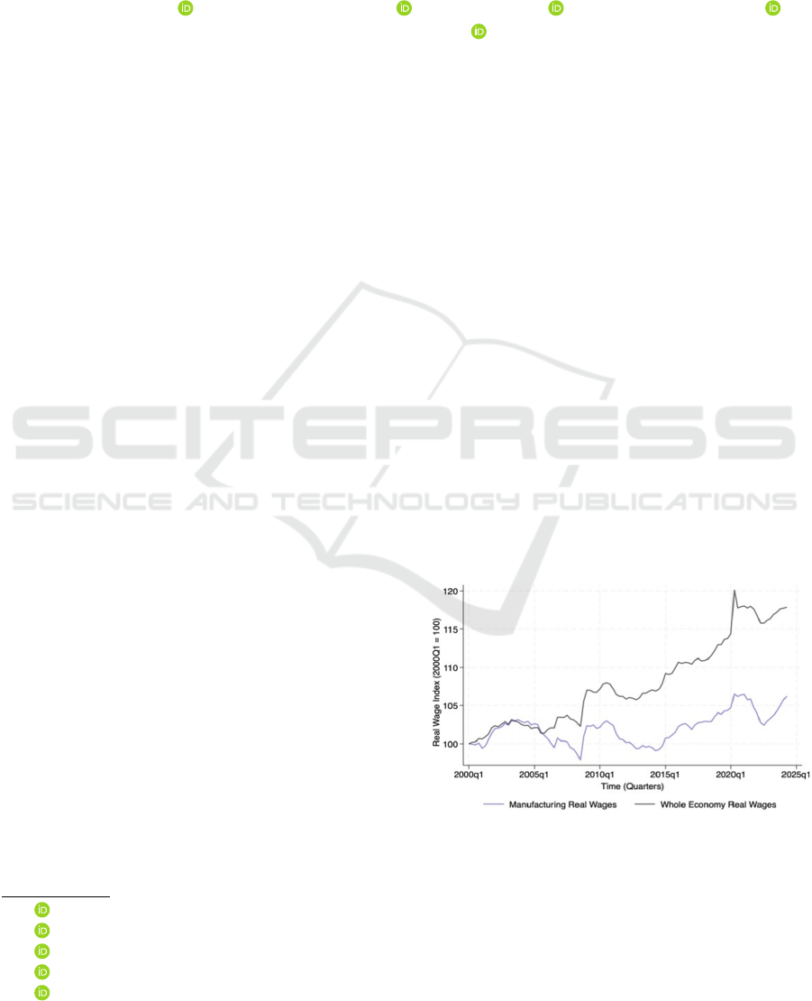
Figure 1: Time Series of Real Wages in the Manufacturing
Sector against Real Wages in the Whole Economy.
ployment in the manufacturing sector has fallen over
the recent decades, its share of GDP has remained
largely constant due to improvements in productiv-
ity (Baily and Bosworth, 2014). This means that the
manufacturing sector has broadly maintained its eco-
nomic relevance throughout this period.
296
Kshirsagar, I., Simon, J. M., Schätz, N., Fraga Gonzalez, D. and Ryan, C.
A Vector Autoregression Model for Depicting the Relation Between Labour Market Economic Indicators and Real Wages in the United States Manufacturing Sector.
DOI: 10.5220/0013123000003890
Paper published under CC license (CC BY-NC-ND 4.0)
In Proceedings of the 17th International Conference on Agents and Artificial Intelligence (ICAART 2025) - Volume 3, pages 296-302
ISBN: 978-989-758-737-5; ISSN: 2184-433X
Proceedings Copyright © 2025 by SCITEPRESS – Science and Technology Publications, Lda.

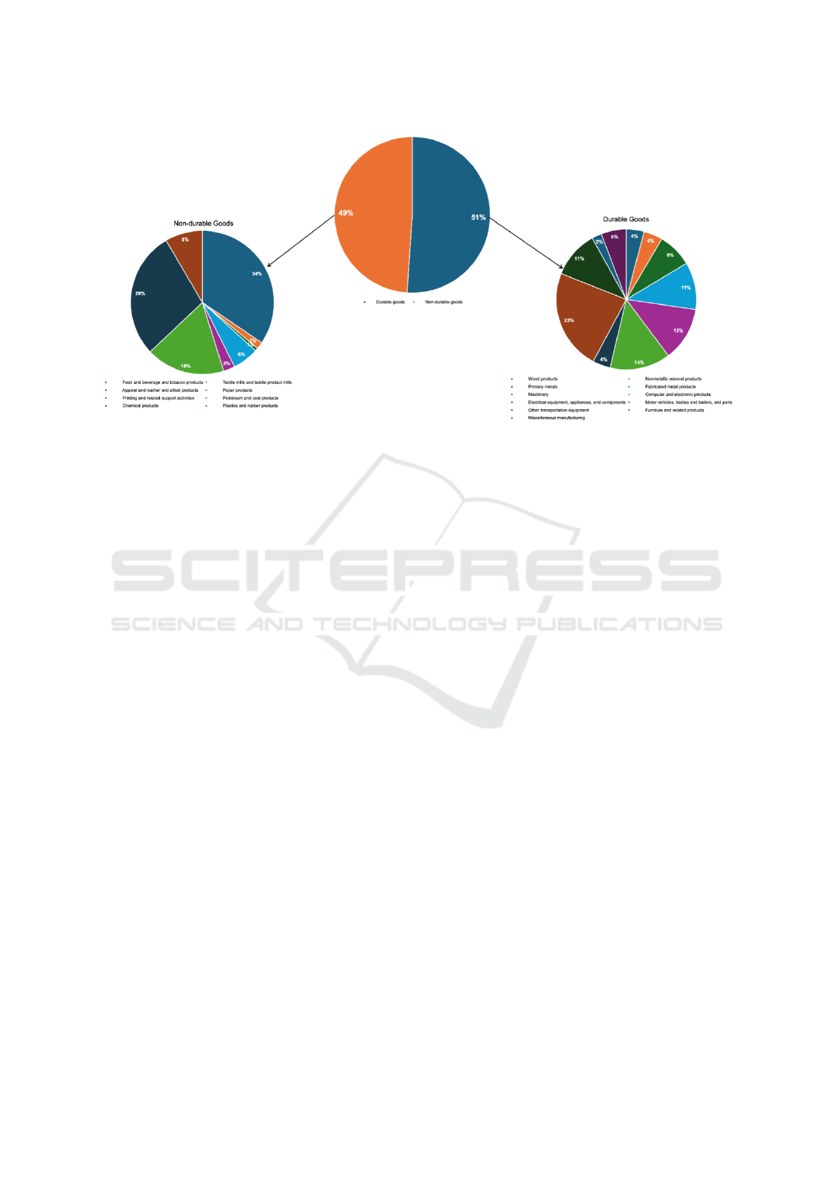
Figure 2: Time Series of Real Wages in the Manufacturing Sector against Real Wages in the Whole Economy.
Additionally, there has been a divergence between
real wages in the manufacturing sector and those
in the wider economy in recent decades (Figure 1).
These factors motivate a fresh analysis of wage de-
termination in the sector. Figure 2 provides insight
regarding the composition of the US manufacturing
sector. The industries shown are the subjects of anal-
ysis for this study.
The literary basis of our study will be further
expanded in Section 2. Section 3 will outline the
methodology, and the variables selected. Section 4
presents the results, visualisations and accompanying
economic discussions followed by the conclusions.
2 LITERATURE REVIEW
The role of labour market variables as determinants
of real wages has been widely discussed in economic
literature. Domash and Summers (2022) utilised job
openings and unemployment rates as indicators of
slackness in the labour market, on the demand and
supply side respectively. To further measure demand
and supply side labour market forces, overtime hours
and industrial production are considered. On the other
hand, capacity utilisation has been employed by Stock
and Watson (2020) to capture real cyclical economic
activity.
A sectoral differentiation of wage determination
has been previously studied by Sheffield (2013). They
utilised a log-transformed linear regression model to
analyse the impact of sector-specific market variables
on real wage growth. The approach taken by Domash
and Summers (2022) relies on various wage Phillips
curve regressions at both the national and state levels
in the US.
Another statistical model that has been utilised to
analyse the effects of a variety of variables on real
wage growth in the past is VAR. Bernanke and Blin-
der (1992) employ a VAR model to determine the ef-
fects of monetary policy on real wages. Similarly,
Blanchard and Quah (1989) employ a structural VAR
to analyse the effects of demand and supply shock
on real wage growth. In both instances, analysis of
the relationship between their chosen macroeconomic
variables and real wage change. However, a VAR
analysis of the manufacturing sector in the US has,
to our knowledge, not been conducted before.
3 METHODOLOGY
This section describes the manufacturing sector’s
labour market variables for the study (Table 1). It also
provides the specifications of the VAR model and the
relevance of utilising VAR.
3.1 Dataset Details
This study uses a curated dataset utilising monthly
data from December 2000 to May 2024 collected
from the Bureau of Labour Statistics (BLS) (2024)
and the Board of Governors of the Federal Re-
serve System via the Federal Reserve Economic Data
(FRED) (2024) to analyse and examine the relation-
ship between real wage change and various labour
market economic indicators.
A Vector Autoregression Model for Depicting the Relation Between Labour Market Economic Indicators and Real Wages in the United
States Manufacturing Sector
297

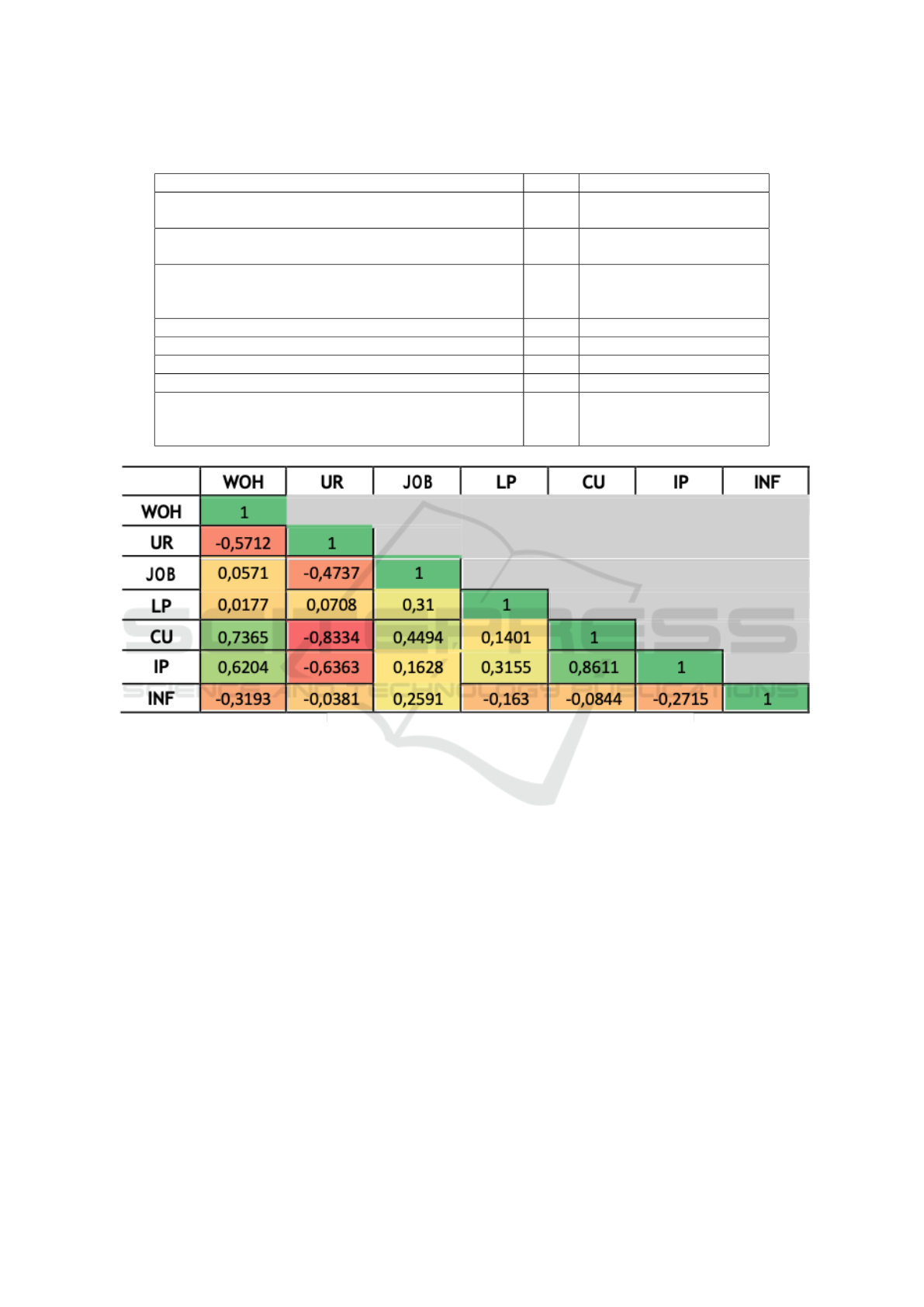
Table 1: Description of Variables.
Variable Code Unit
Year-on-year Change in Real Average Hourly Earnings
of Production and Nonsupervisory Employees
RW Percentage (%)
Avg. Weekly Overtime Hours of Production
and Nonsupervisory Employees
WOH Hours
Unemployment Rate – Private Wage and Salary
Workers
UR Percentage (%)
Job Openings (First Differenced) JOB Rate
Real Sectoral Output for All Workers LP Index (January 2017 = 100)
Capacity Utilisation (NAICS) Rate CU Percentage (%)
Industrial Production (NAICS) IP Index (January 2017 = 100)
Year-on-year Change in the Consumer Price Index (CPI)
for All Urban Consumers: All Items in U.S. City
Average (First Differenced)
INF Percentage (%)
Figure 3: Correlation Matrix.
3.2 Vector Autoregression Model
This study employs a standard VAR model as pro-
posed by Breitung and Hamilton (2020) of the fol-
lowing form as defined in Equation 1:
Y
t
= c +
p
∑
i=1
φ
i
Y
t−i
+ ε
t
(1)
where:
Y
t
: The k × 1 vector of endogenous variables at time
t.
c: The k × 1 vector of constants.
φ
i
: The k × k matrix of coefficients for the i-th lag.
ε
t
: The k × 1 vector of error terms at time t.
p: The number of lags in the model.
VAR models are effective at capturing the inter-
connectedness and the interdependent relationships
among various variables. This is important consider-
ing the frequency of correlations in the dataset (Fig-
ure 3). VAR models enable an in- depth quantitative
time-series analysis, which would be particularly use-
ful to highlight the dynamic relationships among the
multiple labour market time series variables. A 24-
month lag was used to allow economic conditions to
fully reflect on wages. Similar lags were estimated by
Domash and Summers (2022).
Following the standard approach to VAR mod-
elling, we tested for linearity, stationarity, interdepen-
dence of variables, lack of co-integration and suffi-
ciently long time series. Our dataset contains monthly
data for just under 24 years and includes 282 data
points per variable, ensuring that the time-series is
sufficiently long. Furthermore, stationarity was tested
by conducting the ‘Augmented Dickey–Fuller unit-
root test’, which determined that both the job open-
ings rate and year-on-year inflation rate were non-
stationary. To remedy this, a first-differenced trans-
formation for these variables was undertaken, result-
ing in them becoming stationary. Moreover, the ‘Jo-
hansen test for cointegration’ and the ‘LM test for
ICAART 2025 - 17th International Conference on Agents and Artificial Intelligence
298

Table 2: Regression Results with Lagged Variables.
Variable Lag Month Coefficient
Std.
Error
z-value p >z 95% Confidence Interval
Unemployment
Rate Sectoral
24 -0.0822 0.0317 -2.59 0.010 -1.4433 -0.02
Manufacturing Sector
Labour Productivity
24 0.1484 0.0447 3.32 0.001 0.0608 0.2359
Industrial
Production
24 1.2382 0.4125 3.00 0.003 0.4298 2.0466
(First Differenced)
Job Openings Rate
24 0.3116 0.0792 3.94 — 0.1565 0.4668
Average
Overtime Hours
24 -1.6491 0.2122 -7.77 0.000 -2.0649 -1.2332
YOY CPI
(First Difference)
1 -0.7148 0.0964 -7.42 0.000 -0.9036 -0.5259
Capacity
Utilisation Rate
24 -1.5795 0.5203 -3.04 0.002 -2.5992 -0.5597
residual autocorrelation’ were conducted to ensure
that there is no cointegration and no autocorrelation
among selected variables. In addition, the ‘Granger
causality test’ was conducted to check whether there
is Granger Causation between year-on-year (YOY)
change in real wages and the selected labour market
variables. The results of all the Granger causality tests
were significant, reflecting Granger causality between
changes in real wages and our selected labour market
indicators.
Additionally, we have employed a structural break
from November 2008 to October 2009 which covers
the period of volatility and instability during the fi-
nancial crisis and shields our model from parameter
instability at the time. The breakdown in the relation-
ship between labour market variables over this time
period, as evidenced by Michaillat and Saez (2019),
is further supported by our structural break testing us-
ing the algorithm proposed by Bai and Perron (1998,
2003).
4 RESULTS AND DISCUSSIONS
The results from the vector autoregression are shown
in the following Equation 2:
RW = −1.65W OH −0.08UR+ 0.31 JOB+ 0.15 LP
− 1.58CU + 1.24 IP − 0.71 INF + 128.43 (2)
The coefficients above (Table 2) should be inter-
preted as follows: Unemployment rate sectoral indi-
cates that a change in the rate of 1 percentage point is
correlated with a fall of 0.0822 percentage points in
the YOY change in Real Wages in the manufacturing
sector after 24 months. The coefficients of the other
variables can be interpreted in a similar way. The co-
efficient of variables for which the first difference was
taken must be integrated upon interpretation. Figures
4 supplement the results by providing a more time
sensitive dissection of variable comovements across
the analysed period in the form of time series graphs
plotting explanatory variables against YOY change in
Real Wages.
This section will examine the results of the VAR
model using economic theory. According to classical
economic theory, real wage can be determined and af-
fected by various factors such as bargaining power, an
increase in demand for workers, productivity, an in-
crease in the cost of living and inflation, etc. The vari-
ables selected in the VAR model seek to cover these
wage-determining factors.
The negative relationship between the unemploy-
ment rate and real wages may be explained by a re-
duction in worker bargaining power caused by an in-
crease in unemployment. As increases in jobseekers
saturate the labour market, downward pressure is cre-
ated on real wages (Figure 5). Notwithstanding, our
model shows this negative relationship to be relatively
weak. A potential explanation is that workers who
have lost their jobs (and therefore their wages) are ex-
cluded from the average real wage calculation. If the
group of workers which has become unemployed had
lower wages than average, as was observed during the
covid-19 pandemic (Bateman and Ross, 2021), then
real wages would rise ceteris paribus. This may have
partly offset the decrease in real wages due to lower
worker bargaining power, making the coefficient for
the impact of the unemployment rate on real wage rel-
atively smaller than expected.
Similarly, an increase in real wages due to an in-
crease in job openings can be justified due to an in-
A Vector Autoregression Model for Depicting the Relation Between Labour Market Economic Indicators and Real Wages in the United
States Manufacturing Sector
299

Figure 4: Time series graphs of lagged indicators with structural breaks.
Figure 5: Effect of shift in demand for workers.
crease in demand for workers. Industrial production
follows the same trend, given that increasing output
tends to require an increase in workers operating at
a firm. This creates a higher demand for workers,
which increases their bargaining power and subse-
quently, their real wages. Figures 4c and 4f show that
this link looks to remain resilient during times of cri-
sis as can be seen in the coinciding shocks during the
COVID-19 pandemic.
Figure 6: Effect of shift in demand for workers.
Another important factor that determines real
wages is inflation or cost of living. Real wages are de-
rived from the division of nominal wages by the infla-
ICAART 2025 - 17th International Conference on Agents and Artificial Intelligence
300

tion rate, commonly measured by the CPI, as shown
below.
RealWageRate =

NominalWageRate
CPI

× 100 (3)
According to Equation 3, an increase in CPI leads
to a fall in real wages, ceteris paribus. The negative
CPI coefficient from our results implies that wages
have not kept up with inflation over the analysed pe-
riod. This phenomenon looks to be most apparent
during the period of high inflation volatility of the
early 2020s, which was mirrored by large swings in
the YOY change of real wages (as observed in Fig-
ure 4d). This indicates that US manufacturing sec-
tor labour markets struggle to keep pace in uncertain
inflationary environments. Further adding to the de-
pressive effect on real wages is that inflation generally
indicates economic instability, during which invest-
ments in the economy tend to fall as ROI (return on
investment) becomes more uncertain and difficult to
project.
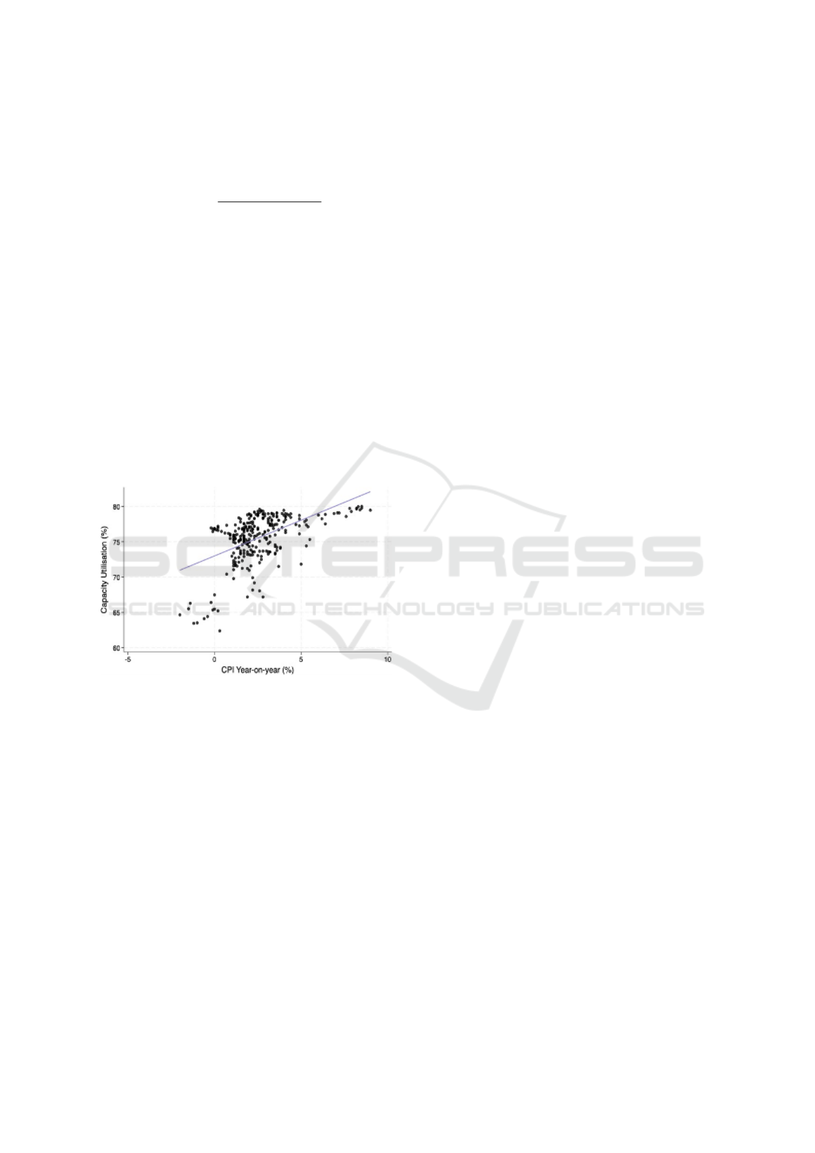
Figure 7: Effect of shift in demand for workers.
The strong negative relationship between average
overtime hours and real wages evidenced by both the
results from the VAR and the synchronous movement
observed in Figure 4e, may be explained by work-
ers choosing to increase their overtime hours during
times of poor economic outlook and high cost of liv-
ing in an effort to maintain their living standards (Ci-
phr, 2023).
The strongly negative coefficient of capacity util-
isation follows orthodox Keynesian economic theory.
As the economy approaches full capacity, an increase
in aggregate demand leads to high inflationary pres-
sure and a decreasing marginal increase in real output
(represented in Figure 6). As previously discussed,
real wages tend to fall under higher inflation. Hence,
ceteris paribus, high-capacity utilisation creates infla-
tionary pressure in an economy, hence lowering real
wages as per Equation (3).
Empirically, the positive relationship between ca-
pacity utilisation and the inflation rate is shown by a
correlation coefficient of 0.42 (See Figure 7).
5 CONCLUSIONS
This research study shows that labour market eco-
nomic conditions are conducive to real wage changes
in the United States’ manufacturing sector between
the years 2000 and 2024.
The study found that the two main factors affect-
ing change in real wages are bargaining power and in-
flation. This is due to an increase in bargaining power
affecting a worker’s ability to negotiate a higher wage
ceteris paribus. In addition, inflation reduces the real
value of a worker’s nominal wage, hence having a sig-
nificant impact on their real wages. By developing a
comprehensive VAR model, this study has displayed
and quantified each lagged variables’ effect on YOY
change in real wages. The dataset and VAR model
results have been presented using a variety of visu-
alisation techniques, including time-series graphs, pie
charts, a scatter plot and heat map. The results are also
significant from a policy perspective. Inflation has
been shown to be highly corrosive to real wages in the
US manufacturing sector as labour markets have not
exhibited sufficient flexibility to absorb the effects.
While it is evident that policy makers ought to pri-
oritise inflation stabilisation, the results from average
overtime hours indicate that certain contractionary fis-
cal policies may not be effective in periods of eco-
nomic overheating. For example, income taxation
would not efficiently reduce aggregate demand (a key
factor in the reduction of inflation) as the results sug-
gest workers prefer to increase working hours rather
than decreasing personal consumption.
The approach taken in this paper could be ex-
panded to include other sectors or countries in future
studies.
ACKNOWLEDGEMENTS
We are grateful to Dr Monika Sosa Smatralova for her
valuable insights.
REFERENCES
Bai, J. and Perron, P. (1998). Estimating and testing linear
models with multiple structural changes. Economet-
rica, 66(1):47.
A Vector Autoregression Model for Depicting the Relation Between Labour Market Economic Indicators and Real Wages in the United
States Manufacturing Sector
301

Bai, J. and Perron, P. (2003). Computation and analysis of
multiple structural change models. Journal of Applied
Econometrics, 18(1):1–22.
Baily, M. N. and Bosworth, B. P. (2014). Us manufacturing:
Understanding its past and its potential future. Journal
of Economic Perspectives, 28(1):3–26.
Bateman, N. and Ross, M. (2021). The pandemic
hurt low-wage workers the most—and so
far, the recovery has helped them the least.
Retrieved from https://www.brookings.edu/
articles/\\the-pandemic-hurt-low-wage-workers\
\-the-most-and-so-far-the-recovery\
\-has-helped-them-the-least/.
Bernanke, B. S. and Blinder, A. S. (1992). The federal funds
rate and the channels of monetary transmission. The
American Economic Review, 82(4):901–921. [online].
Blanchard, O. J. and Quah, D. T. (1989). The dynamic ef-
fects of aggregate demand and supply disturbances.
The American Economic Review, 79(4):655–673.
Available at: http://www.jstor.org/stable/1827924.
Breitung, J. and Hamilton, J. D. (2020). Time series analy-
sis. Contemporary Sociology, 24(2):271.
Ciphr (2023). Two in five employees are working
extra hours as cost-of-living crisis bites. Re-
trieved from https://www.ciphr.com/press-releases/
\\two-in-five-employees-are-working-extra\
\-hours-as-cost-of-living-crisis-bite/.
Domash, A. and Summers, L. (2022). A labor market view
on the risks of a u.s. hard landing.
Federal Reserve Economic Data . Federal reserve economic
data — fred — st. louis fed. https://fred.stlouisfed.org.
[Accessed 19-12-2024].
Michaillat, P. and Saez, E. (2019). Beveridgean unemploy-
ment gap. NBER Working Paper. https://www.nber.
org/papers/w26474.
Sheffield, J. (2013). Contending theories of wage determi-
nation: An intersectoral analysis of real wage growth
in the u.s. economy. Pursuit: The Journal of Un-
dergraduate Research at the University of Tennessee,
4(2):4.
Stock, J. H. and Watson, M. W. (2020). Slack and cycli-
cally sensitive inflation. Journal of Money, Credit and
Banking, 52(S2):393–428.
U.S. Bureau of Labor Statistics. U.s. bureau of labor Statis-
tics. https://www.bls.gov/. [Accessed 19-12-2024].
ICAART 2025 - 17th International Conference on Agents and Artificial Intelligence
302