Latent Space Characterization of Autoencoder Variants

Anika Shrivastava

, Renu Rameshan

2 a

and Samar Agnihotri

1,2 b

School of Computing and EE, IIT Mandi, HP - 175005, India

Vehant Technologies Pvt. Ltd., UP - 201301, India

Keywords:

Representation Learning, Autoencoder, Latent Space, Hilbert Space, Matrix Manifold.

Abstract:

Understanding the latent spaces learned by deep learning models is crucial in exploring how they represent

and generate complex data. Autoencoders (AEs) have played a key role in the area of representation learning,

with numerous regularization techniques and training principles developed not only to enhance their ability to

learn compact and robust representations, but also to reveal how different architectures inﬂuence the structure

and smoothness of the lower-dimensional non-linear manifold. We strive to characterize the structure of

the latent spaces learned by different autoencoders including convolutional autoencoders (CAEs), denoising

autoencoders (DAEs), and variational autoencoders (VAEs) and how they change with the perturbations in the

input. By characterizing the matrix manifolds corresponding to the latent spaces, we provide an explanation

for the well-known observation that the latent spaces of CAE and DAE form non-smooth manifolds, while

that of VAE forms a smooth manifold. We also map the points of the matrix manifold to a Hilbert space

using distance preserving transforms and provide an alternate view in terms of the subspaces generated in the

Hilbert space as a function of the distortion in the input. The results show that the latent manifolds of CAE

and DAE are stratiﬁed with each stratum being a smooth product manifold, while the manifold of VAE is a

smooth product manifold of two symmetric positive deﬁnite matrices and a symmetric positive semi-deﬁnite

matrix.

1 INTRODUCTION

With the emergence of cutting-edge deep learning

models, the ﬁeld of image processing has seen sig-

niﬁcant progress. However, this advancement neces-

sitates a deeper understanding of the inner workings

of these models, speciﬁcally how they represent data.

Autoencoders, introduced in (Rumelhart et al., 1986),

serve as the foundation for a wide range of unsuper-

vised learning models (Zhai et al., 2018) and have

gained signiﬁcant attention for their ability to learn

meaningful representations of data. They learn these

representations with the help of a simple end-to-end

structure involving two main components: an encoder

and a decoder. The input y ∈ R

is mapped to a

latent representation z ∈ R

via an encoding func-

tion f : R

→ R

, and then the decoder reconstructs

it back in the original space using a decoding func-

tion g : R

→ R

, minimizing the reconstruction loss

L(y,

y), where y is the original input and

y is its re-

construction. In essence, the latent space is where z

lies. Characterizing the latent space involves analyz-

https://orcid.org/0000-0002-7623-0510

https://orcid.org/0000-0003-3038-2479

ing how autoencoders arrange data within this space,

understanding the properties of this space, and assess-

ing whether smooth navigation is possible within the

space. We believe that knowing the structure of the la-

tent space can guide one in designing better restoration

algorithms.

Traditionally, autoencoders are introduced as a di-

mensionality reduction technique, where the latent

space has a dimension d < D, resulting in an under-

complete autoencoder. This dimensionality restric-

tion acts as a form of regularization, forcing the model

to learn only the most important features of y. How-

ever, some variants of autoencoders, known as over-

complete autoencoders, employ latent spaces with di-

mensions equal to or even larger than the input space.

While this design has the potential to capture the clos-

est reconstruction of the input image, it also intro-

duces the risk of the model learning an identity func-

tion (Bengio et al., 2013), where it simply replicates

the input, thus failing to learn any useful representa-

tions. To prevent this, over-complete models are of-

ten combined with regularization techniques such as

weight decay, adding noise to input images (Vincent

et al., 2008), imposing sparsity constraints (Ng et al.,

Shrivastava, A., Rameshan, R. and Agnihotri, S.

Latent Space Characterization of Autoencoder Variants.

DOI: 10.5220/0013123700003912

Paper published under CC license (CC BY-NC-ND 4.0)

In Proceedings of the 20th International Joint Conference on Computer Vision, Imaging and Computer Graphics Theory and Applications (VISIGRAPP 2025) - Volume 2: VISAPP, pages

59-67

ISBN: 978-989-758-728-3; ISSN: 2184-4321

2011), or by adding a penalty term to the loss func-

tion to make the space contractive (Rifai et al., 2011).

These regularizations help in structuring the latent

space to be compact and robust against small varia-

tions in the input data, enabling the model to learn ro-

bust and meaningful patterns rather than merely copy-

ing the input. Additionally, some variants introduce

a stochastic component by enforcing a probabilistic

latent space, which ensures smooth latent manifold

leading to better generalization (Kingma and Welling,

2013). In Section 2, we discuss how these regulariza-

tion methods shape the properties of the latent space.

However, while these methods impose some structure

on the latent space, they do not directly explain the

underlying manifold—speciﬁcally, its geometry and

properties. Our work aims to bridge this gap by pro-

viding a more detailed understanding of the manifold

structure learned by different autoencoder variants.

We aim to characterize the latent spaces of over-

complete Convolutional autoencoders (CAE), De-

noising autoecnoders (DAE), and Variational au-

toencoders (VAE) by analyzing how varying levels

of noise impact their respective learned latent mani-

folds and whether the structures of these spaces per-

mit smooth movement within them. Empirically, it

is observed that autoencoders exhibit a non-smooth

latent structure (Oring, 2021), while VAEs tend to

have a smooth latent structure (Cristovao et al., 2020).

A simple experiment to visually illustrate this differ-

ence involves interpolating between two data points

by decoding convex combinations of their latent vec-

tors (Berthelot et al., 2018). For CAE and DAE, this

often leads to artifacts or unrelated output, indicating

the lack of smooth transitions between the two points.

In contrast, VAE exhibits a coherent and smooth tran-

sition, reﬂecting its continuous latent space. Our ap-

proach builds upon the work of (Sharma and Rame-

shan, 2021), where video tensors are modeled as

points on the product manifold (PM) formed by the

Cartesian product of symmetric positive semi-deﬁnite

(SPSD) matrix manifolds. We adapt this method for

the encoded tensors extracted from each model’s la-

tent space and examine the ranks of the SPSD matri-

ces to analyze the structure of the learned latent man-

ifold. This analysis provides support for the fact that

the latent spaces of CAE and DAE have non-smooth

structure as those are stratiﬁed manifolds with each

stratum being a smooth manifold based on the ranks,

while that of the VAE forms a smooth product mani-

fold of SPD and SPSD matrices. Further, we trans-

form these PM points to the Hilbert space using a

distance based positive-deﬁnite kernel (Sharma and

Rameshan, 2021), allowing us to analyze the latent

spaces in terms of subspaces.

Our main contribution is in characterizing the

manifold by using a simple observation namely, the

latent tensors lie on a product manifold of symmet-

ric positive semideﬁnite matrices. We also explore

how the manifold structure changes with perturba-

tions in the input. Perturbations are modeled by ad-

ditive white Gaussian noise with different variances.

We show that while CAE and DAE have a stratiﬁed

matrix manifold, VAE has a matrix manifold that is

smooth.

Organization: The remainder of the paper is struc-

tured as follows. Section 2 provides a brief literature

review. Section 3 discusses the approach used for the

characterization of latent spaces, followed by exper-

imental details in Section 4. Section 5 analyzes the

results obtained and discussed their various implica-

tions. Finally, Section 6 concludes the paper and pro-

vides some directions for the future work.

2 RELATED WORK

Regularization-Guided Latent Spaces. The widely

recognized manifold hypothesis (Fefferman et al.,

2016) suggests that a ﬁnite set of high dimen-

sional data points concentrate near or on a lower-

dimensional manifold M . A manifold is basically

a topological space that locally resembles Euclidean

space near each point, and autoencoders are instru-

mental in learning this underlying latent manifold.

Several autoencoder variants employ regularization

techniques to enhance the robustness and structure

of the underlying latent manifold. (Vincent et al.,

2008) introduce Denoising autoencoders (DAEs), a

modiﬁcation to the traditional autoencoders where

the model learns to reconstruct clean images ˆy from

noisy/corrupted inputs ˜y, thereby, minimizing the re-

construction loss L (y, ˆy). From a manifold learning

perspective, the latent space of DAEs identiﬁes the

lower dimensional manifold where the clean data re-

sides and DAEs learn to map the corrupted data back

onto this manifold. This enables the model to gen-

eralize better, capturing essential latent representa-

tions while being robust to noise. Based on a simi-

lar motive of learning the lower-dimensional manifold

and robust latent representations (Rifai et al., 2011)

add a contractive penalty to the learning process.

Unlike traditional autoencoders, contractive autoen-

coders apply a regularization term to the encoder’s

Jacobian matrix, penalizing the sensitivity of the la-

tent space to small input changes. In other words,

the underlying latent manifold becomes locally in-

variant to small variations in the input and contracts

the latent space along these directions of unimportant

VISAPP 2025 - 20th International Conference on Computer Vision Theory and Applications

output

input

Skip-connected Triple convolution (SCTC)

Convolution layers with

same no. of filters

Input

image

Latent

tensor

256

output

image

128

32 64

128

7x7x256

7x7x128

128 64

Feature extraction Reconstruction

SCTC block with

Conv layers

Maxpool layer Feature maps

Single Conv layer

SCTC block with

Conv transpose

layers

Concatenate

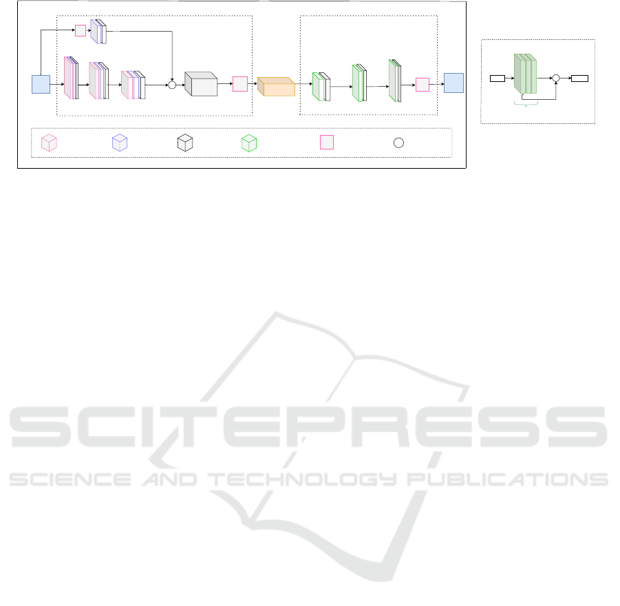
Figure 1: The SCTC block used in CAE and DAE models.

variations. Similarly, sparse autoencoders (Ng et al.,

2011) learn non-redundant representations by enforc-

ing sparsity in the hidden units. By activating only

a few neurons at a time, the model captures more

distinct, disentangled features, resulting in a sparse,

interpretable and efﬁcient latent space. In addition

to these techniques, Variational autoencoders (VAEs)

(Doersch, 2016) introduce a probabilistic structure to

the latent space by learning a distribution over the la-

tent variables, rather than representing them as ﬁxed

points. This pushes the latent space toward being con-

tinuous and smooth, facilitating tasks like data gener-

ation and interpolation.

Representation Geometry. Several studies explore

and regularize the geometry of the latent represen-

tation in VAEs. For instance, (Chadebec and Allas-

sonnière, 2022) show that the latent manifold learned

by VAEs can be modeled as a Riemannian manifold,

while (Chen et al., 2020) extend the VAE framework

to learn ﬂat latent manifolds by regularizing the met-

ric tensor to be a scaled identity matrix. (Connor

et al., 2021) incorporate a learnable manifold model

into the latent space to bring the prior distribution

closer to the true data manifold. Additionally, (Leeb

et al., 2022) develop tools to exploit the locally con-

tractive behaviour of VAEs to better understand the

learned manifold. These and many other studies as-

sume that VAEs learn a smooth manifold, whereas

AEs learn a non-smooth manifold (Oring, 2021), but

the exact structure and properties of these manifolds

have not been thoroughly explored.

We aim to capture the precise structure of the la-

tent space and how it evolves when processing images

with varying levels of noise. Our results conﬁrm that

the latent manifolds learned by AEs are non-smooth,

while the manifold learned by VAEs is smooth - ex-

plaining the reasons behind this behavior and char-

acterizing the space in detail. Many studies have

demonstrated the effectiveness of modeling sample

data as points in the product manifold across various

vision tasks (Abdelkader et al., 2011; Lui et al., 2010;

Lui, 2012; Sharma and Rameshan, 2019). Motivated

by this, we strive to thoroughly model the latent space

points in the PM of the SPSD matrices to characterize

the behaviour of latent spaces of different models.

3 PRODUCT MANIFOLD

STRUCTURE

In this section, we describe the details of the au-

toencoder network used for feature extraction and the

method we adopt for modeling the encoded latent ten-

sors as points in the PM of SPSD matrices, and for

further transforming PM points to the Hilbert space.

3.1 Model Architectures

The architecture used for extracting latent tensors

in both CAE and DAE models is built of "Skip-

Connected Triple Convolution” (SCTC) block as

shown in Fig. 1. Each SCTC block contains three

convolutional layers with the same number of ﬁlters

and a skip connection from the ﬁrst convolution to the

third convolution. The encoder is composed of three

such layers, each followed by max-pooling. Addi-

tionally, a skip connection is introduced directly from

the input image to the latent representation using a

single convolutional and max-pooling layer. The de-

coder mirrors the encoder’s structure, using the SCTC

blocks with transpose convolution layers to recon-

struct the images from the latent tensor. We select the

SCTC blocks after extensive experimentation. To as-

sess the impact of the SCTC blocks, we replace them

with standard convolution layers, which result in re-

duced PSNR, conﬁrming their importance in preserv-

ing image details. Additionally, removing the direct

skip connection from the input to the latent tensor

again leads to a drop in PSNR, underscoring its role

in better feature retention.

For VAEs, we use a standard convolutional VAE

architecture. However, instead of using linear layers

Latent Space Characterization of Autoencoder Variants

Encoder

Input

images

Encoded latent tensor

for each image

Latent tensor

decomposition

Each encoded

latent tensor

Matrix unfolding

operation

Product of

SPSD matrices

Product Manifold

Hilbert Space

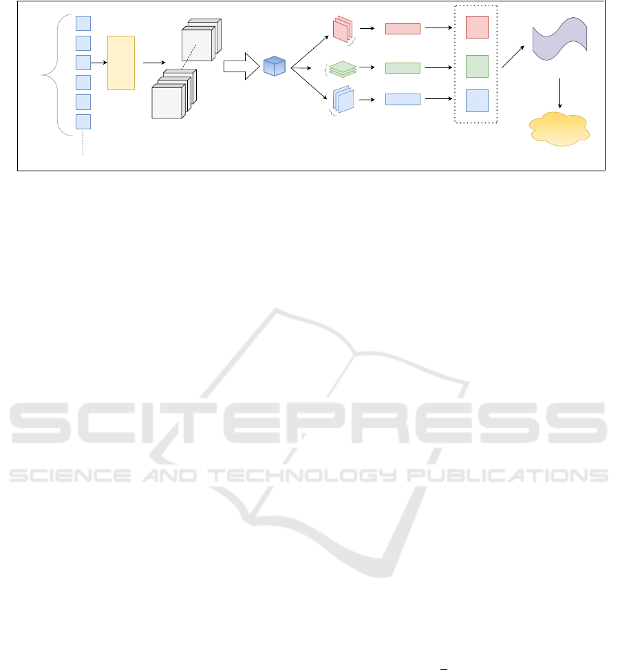
Figure 2: Pipeline of the proposed approach.

to compute the mean (µ) and log variance, we employ

convolution layers to generate a latent tensor instead

of a latent vector. Through experimentation, we con-

ﬁrm that both latent vectors and latent tensors yield

similar reconstruction output. Based on this, we opt

for latent tensors to maintain consistency, with the

shape of the extracted latent tensor ﬁxed at 7×7×128

for all models to ensure fair comparison.

3.2 Latent Tensors as Points in a

Product Manifold

The encoded latent tensors can be understood as

points lying on a PM of the SPSD matrices. An il-

lustration of the pipeline used for representing en-

coded latent tensors as points in the PM of the SPSD

matrices is shown in Fig. 2 (inspired by (Sharma

and Rameshan, 2021)). Let the encoded feature ten-

sors have the shape (N, n

, n

), where N repre-

sents the number of test samples. Each feature tensor

can be interpreted as a point F ∈ R

×n

, with n

and n

corresponding to height, width, and num-

ber of channels of the encoded image, respectively.

These tensors are then decomposed into a set of three

matrices F 7→ {F

(1)

, F

(2)

, F

(3)

}, using matrix unfold-

ing, where F

(1)

∈ R

×(n

·n

)

, F

(2)

∈ R

×(n

·n

)

, and

(3)

∈ R

×(n

·n

)

. For each F

(i)

, a covariance matrix

is calculated denoted as S

(1)

, S

(2)

, S

(3)

and these are

inherently the SPSD matrices. The Cartesian product

of these covariance matrices is a product manifold of

the SPSD manifolds (Rodolà et al., 2019).

By deﬁnition, the SPSD manifold S

(r)

(Bonnabel and Sepulchre, 2010) is the space of

n × n SPSD matrices of ﬁxed rank r. The SPSD

matrices sharing the same rank belong to the same

manifold. The collection of all n × n SPSD matrices

with rank ≤ r is not a manifold. It is well known

that the collection of all n × n SPSD matrices with

varying ranks, forms a stratiﬁed manifold (Massart

et al., 2019). The ranks r

, r

of the matrices

(1)

, S

(2)

, S

(3)

, respectively, form a tuple (r

, r

characterizing the overall rank conﬁguration of the

latent tensor within the PM. We show in Section 5

that the way this rank tuple behaves with varying

noise levels is different for the three architectures.

The variability in these ranks indicate whether the

underlying manifold is smooth or stratiﬁed.

3.3 Transformation to Hilbert Space

To simplify the understanding, instead of viewing the

latent representation as a tensor in the SPSD mani-

fold, we adopt an alternative approach by embedding

these points into a Hilbert space. Each covariance de-

scriptor S

(i)

is regularized to a ﬁxed rank r

by replac-

ing zero eigenvalues with small epsilon value, where

corresponds to the maximum rank observed across

all test samples for each i ∈ {1, 2, 3}. The decomposi-

tion of each S

(i)

is given as (Bonnabel and Sepulchre,

2010):

(i)

= A

(i)

(i)⊤

= (U

(i)

)(U

(i)

)

⊤

(i)

(i)2

(i)⊤

for i ∈ {1, 2, 3} corresponding to each unfolding.

Here, U ∈ R

n×r

has orthonormal columns; n is the

size of S and r its rank. R is an SPD matrix of

size r. Following (Sharma and Rameshan, 2021), the

geodesic distance function between any two points

, γ

on the PM of the SPSD matrices is deﬁned as:

(γ

, γ

) =

∑

i=1

∥U

(i)

(i)T

−U

(i)

(i)T

∥

+λ

(i)

∥log(R

(i)

) − log(R

(i)

)∥

(1)

For further analysis, we use the positive deﬁnite

linear kernel function that follows from Eq. 1:

lin

(γ

, γ

) =

∑

i=1

∥U

(i)T

(i)

∥

+λ

(i)



log(R

(i)

)log(R

(i)

)



(2)

VISAPP 2025 - 20th International Conference on Computer Vision Theory and Applications

where w

denotes the weight for each factor manifold

and tr denotes trace of a matrix. The transformation

from the PM to the Hilbert space is achieved using

this distance based positive deﬁnite kernel function.

It has been shown in (Sharma and Rameshan, 2021)

that such a kernel ensures that the distances between

points in the manifold are maintained in the Hilbert

space after the transformation.

Using the kernel in Eq. 2, we can obtain virtual

features (VF) for each of the data tensor as described

in (Zhang et al., 2012). If there are N data points, then

the virtual feature is a length N vector obtained from

the kernel gram matrix (K) and its diagonalization.

Following the observation that not all the eigenvalues

of K are signiﬁcant, we do a dimensionality reduction

and map the manifold points to a lower dimensional

subspace of R

. In Section 5, we demonstrate how

the dimensionality of the space changes with varying

noise levels for the three autoencoder variants.

4 EXPERIMENTAL SETUP

Training Data. We train our models on the MNIST

dataset. The CAE and VAE models are trained us-

ing 60,000 clean images, while the DAE is trained on

a noisy version of the dataset, with Gaussian noise

(sigma = 0.05) added to the training images.

Testing Data. To effectively capture the changes in

structure of the underlying latent manifold for each

model, we construct a comprehensive test dataset

from the MNIST test set. This dataset includes

multiple classes, each containing 300 images. The

ﬁrst class contains clean images, while the subse-

quent classes are progressively corrupted with Gaus-

sian white noise, with the variance increasing in in-

crements of 0.01.

Training Loss. For the CAE and DAE, we employ

a custom loss function that combines the weighted

sum of MSE and SSIM losses, with equal weights.

For the VAE, we train it using the MSE reconstruc-

tion loss along with the Kullback–Leibler Divergence

loss, where the KLD term is weighted by a parameter

β = 0.8.

5 RESULTS AND ANALYSIS

Empirical observations in the existing literature show

that autoencoders like CAEs and DAEs tend to exhibit

a non-smooth latent structure, while VAEs are known

for producing a smooth latent structure. We aim to

explain this widely discussed hypothesis by explor-

ing what these manifolds exactly are and motivate our

ﬁndings from different perspectives.

5.1 Latent Space Structure in Manifold

Space

In our ﬁrst experiment, we use the Berkeley segmen-

tation dataset (BSDS) to train the CAE and DAE mod-

els. The latent tensor corresponding to each image

in the test dataset is modeled as a point on the PM

formed of the SPSD matrices, as described in subsec-

tion 3.2. S

(1)

, S

(2)

, S

(3)

have shapes 32 × 32, 32 × 32

and 128 × 128, respectively, corresponding to each

unrolled matrix. The ranks of these SPSD matri-

ces are then calculated across different noise levels.

The rank conﬁguration (r

, r

) decides the product

manifold in which the latent tensor lies. It is observed

that all the latent tensors do not lie on the same prod-

uct manifold in the case of CAE and DAE. For clean

images and at lower noise levels, the latent tensors

are distributed across different strata of the product

manifold whereas at higher noise levels they tend to

lie on fewer strata. For a fair comparison between

the three models, we switch to the MNIST data as all

three models present a similar reconstruction perfor-

mance on this dataset. The CAE and DAE exhibit a

behaviour similar to that for the BSDS. Contrary to

this behaviour, the latent tensors of the VAE lie in

the same product manifold for clean as well as for

noisy cases at all noise variances. The rank variablilty

across the three models is given in Fig. 3. The ranks

of the three SPSD matrices for varying noise are pre-

sented in Table 1. These ranks are reported as ranges

(min, max) for each case to reﬂect the observed vari-

ability across the dataset. We observe that the ranks

of the SPSD matrices, mostly S

(3)

, for CAE and DAE

vary across different noise levels, while for VAE, the

corresponding ranks remain ﬁxed.

The variability in the ranks of the SPSD matri-

ces observed in CAE and DAE results in a stratiﬁed

manifold. Since each SPSD matrix lies on a speciﬁc

SPSD manifold deﬁned by its rank, the latent spaces

of the CAE and DAE span multiple product manifolds

determined by the tuple (r

, r

) creating stratiﬁca-

tion of space (Takatsu, 2011). In contrast, the VAE

shows consistent ranks across all noise levels for the

three covariance matrices, indicating that all tensors

lie on the same product manifold - product of two

SPD manifolds and an SPSD manifold. This consis-

tency results in smooth movement within the latent

space from one point to another, describing the latent

space of the VAE as a smooth product manifold.

Latent Space Characterization of Autoencoder Variants

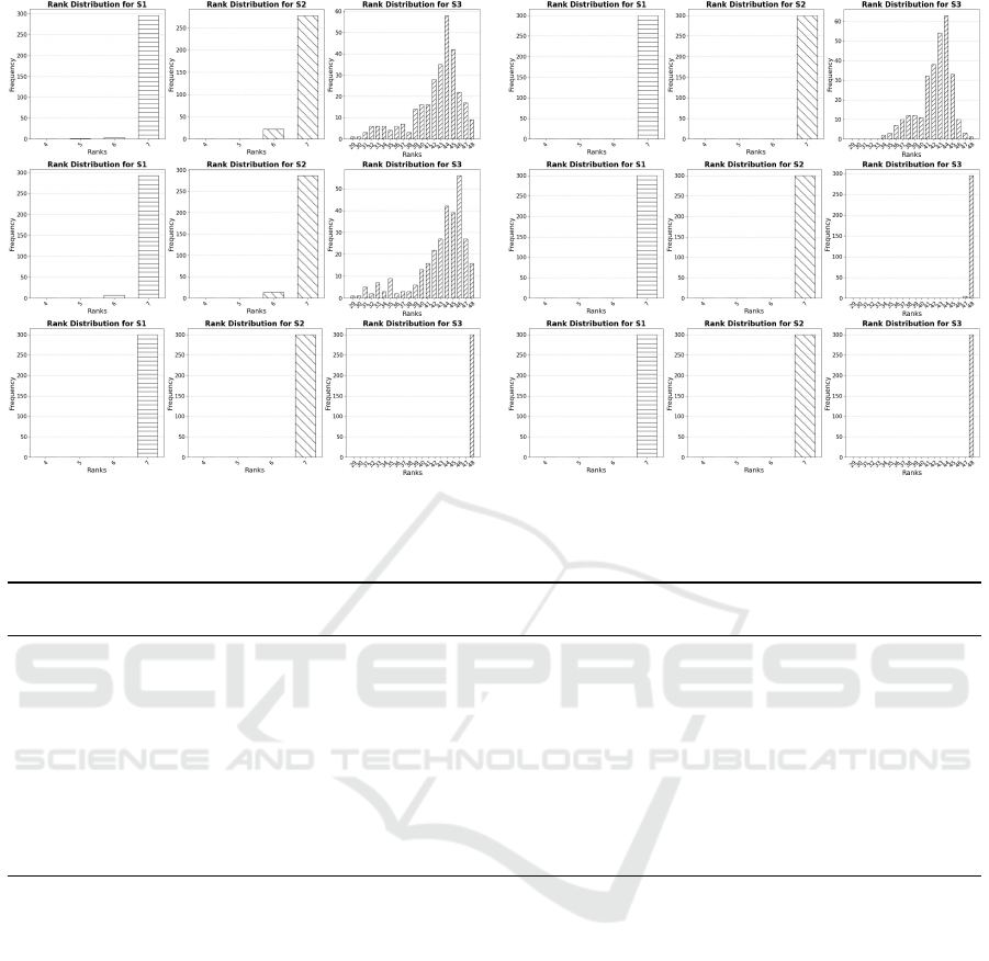
Figure 3: Histograms of ranks of S

(1)

, S

(2)

, S

(3)

for the three models on 300 test samples. Left side is for clean and right for

noisy with standard deviation 0.1. From top to bottom: CAE, DAE, VAE.

Table 1: Ranks of unrolled covariance matrices across different noise level for CAE, DAE, and VAE.

Noise

levels

CAE (latent shape: 7x7x128) DAE (latent shape: 7x7x128) VAE (latent shape: 7x7x128)

zero S1: (5, 7), S2: (6, 7), S3: (29, 48) S1: (6, 7), S2: (6, 7), S3: (29, 48) S1: (7, 7), S2: (7, 7), S3: (48, 48)

0.01 S1: (6, 7), S2: (7, 7), S3: (30, 48) S1: (7, 7), S2: (6, 7), S3: (42, 48) S1: (7, 7), S2: (7, 7), S3: (48, 48)

0.02 S1: (5, 7), S2: (7, 7), S3: (30, 48) S1: (6, 7), S2: (7, 7), S3: (42, 48) S1: (7, 7), S2: (7, 7), S3: (48, 48)

0.03 S1: (6, 7), S2: (7, 7), S3: (32, 48) S1: (6, 7), S2: (7, 7), S3: (42, 48) S1: (7, 7), S2: (7, 7), S3: (48, 48)

0.04 S1: (6, 7), S2: (7, 7), S3: (32, 48) S1: (7, 7), S2: (7, 7), S3: (43, 48) S1: (7, 7), S2: (7, 7), S3: (48, 48)

0.05 S1: (6, 7), S2: (7, 7), S3: (31, 48) S1: (7, 7), S2: (7, 7), S3: (44, 48) S1: (7, 7), S2: (7, 7), S3: (48, 48)

0.06 S1: (7, 7), S2: (7, 7), S3: (31, 48) S1: (7, 7), S2: (7, 7), S3: (43, 48) S1: (7, 7), S2: (7, 7), S3: (48, 48)

0.07 S1: (7, 7), S2: (7, 7), S3: (32, 48) S1: (7, 7), S2: (7, 7), S3: (45, 48) S1: (7, 7), S2: (7, 7), S3: (48, 48)

0.08 S1: (7, 7), S2: (7, 7), S3: (33, 48) S1: (7, 7), S2: (7, 7), S3: (46, 48) S1: (7, 7), S2: (7, 7), S3: (48, 48)

0.09 S1: (7, 7), S2: (7, 7), S3: (33, 48) S1: (7, 7), S2: (7, 7), S3: (47, 48) S1: (7, 7), S2: (7, 7), S3: (48, 48)

0.1 S1: (7, 7), S2: (7, 7), S3: (34, 48) S1: (7, 7), S2: (7, 7), S3: (47, 48) S1: (7, 7), S2: (7, 7), S3: (48, 48)

5.2 Latent Space Structure in Hilbert

Space

The stratiﬁed structure observed in CAE and DAE

can be difﬁcult to visualize directly within the prod-

uct manifold space. Therefore, we transform the PM

points into Hilbert space, as detailed in subsection 3.3.

This is justiﬁed as the distance between the points

are preserved in both the spaces as shown in (Sharma

and Rameshan, 2021). For a test dataset with N data

points, an N ×N kernel-gram matrix is generated. We

proceed by calculating virtual features, followed by

dimensionality reduction to derive N-length vectors

lying on a d-dimensional subspace of R

. The dimen-

sion d for each noise level is determined by minimiz-

ing the difference between the original kernel-gram

matrix and its rank-i approximations and selecting the

smallest i such that the norm falls below a certain

threshold. Fig. 4 illustrates the change in d with noise

levels.

Rather than dealing with multiple product mani-

folds that arise for CAE and DAE, we use a regular-

izer - adding a small value to all the zero eigenvalues

of the SPSD matrices - and push all the points to lie on

a single product manifold. While it may seem that this

simpliﬁcation destroys the structure, our results show

that the rank variability gets reﬂected as variability of

subspace dimension in the Hilbert space.

We observe that for the CAE and DAE, the di-

mensionality of subspaces decreases as the input tran-

sitions from clean to noisy, indicating that the sub-

spaces in the Hilbert space change with increasing

noise. The CAE experiences a sharper drop in dimen-

sionality, while the DAE preserves it slightly better.

In contrast, the VAE points lie in the same subspace

regardless of the noise level.

VISAPP 2025 - 20th International Conference on Computer Vision Theory and Applications

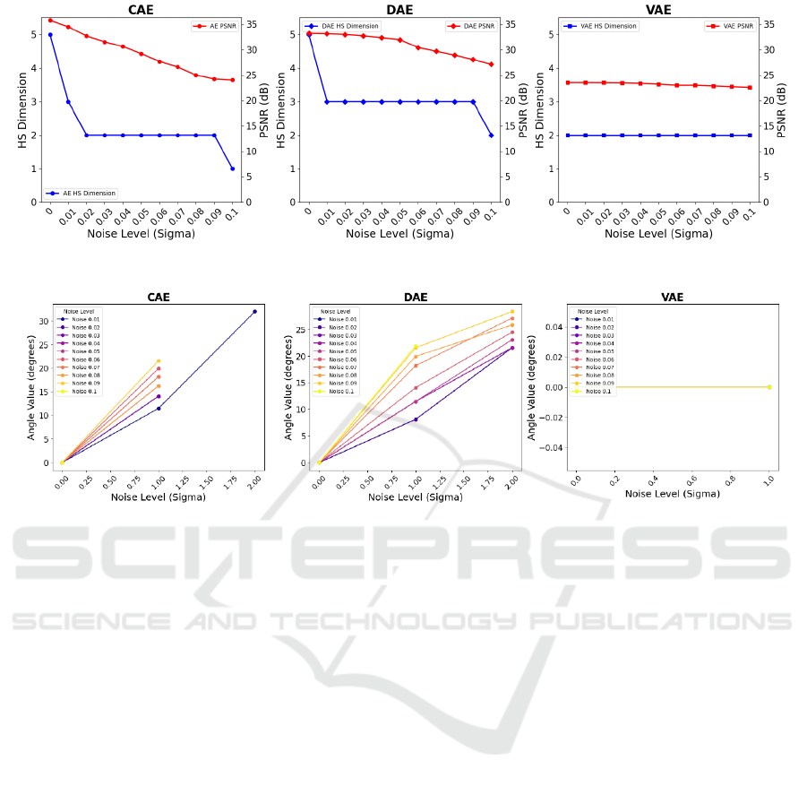
Figure 4: The Hilbert space dimensionality and PSNR versus noise level for CAE, DAE, and VAE.

Figure 5: Principal angle variations for CAE, DAE, VAE.

With noisy subspace dimensions differing from

those of the clean subspace, we have so far estab-

lished that CAE and DAE points lie on distinct sub-

spaces for noisy cases. To examine how the subspaces

corresponding to noisy inputs are oriented with re-

spect to the clean ones, we calculate the principal

angles (Knyazev and Zhu, 2012) between noisy and

clean subspaces at each noise level. Given two sub-

spaces X and X

′

with dimensions d and d

′

, respec-

tively, the number of principal angles is determined by

m = min(d, d

′

). The results, presented in Fig.5, show

that for the CAE and DAE, the principal angles in-

crease with noise level, suggesting that the noisy sub-

spaces diverge away from the clean ones with noise.

This divergence is more pronounced in the CAE. In

contrast, the VAE shows zero principal angles as ex-

pected.

We also examine how PSNR behaves across dif-

ferent noise levels (Fig. 4). It is observed that as

the subspace dimension decreases, the PSNR tends

to drop, particularly in CAE and DAE, whereas VAE

maintains both constant dimensionality and consistent

PSNR across all noise levels, suggesting a connection

between the two.

5.3 Visualizing the Latent Tensors

To provide a clear visual representation of the learned

latent tensors for the three models across different

noise levels, we used t-distributed Stochastic Neigh-

bor Embedding (t-SNE) (Van der Maaten and Hin-

ton, 2008) of the latent tensors extracted from each

model. The t-SNE is a dimensionality reduction tech-

nique that projects high-dimensional data into a two-

dimensional Euclidean space, enabling easier visual

comparison of latent spaces and complementing the

more abstract analysis in the Hilbert space. Fig. 6

shows the t-SNE plots of the ﬂattened latent tensors

for each model across different noise levels, with each

color representing a different noise level and blue dots

denoting the clean images.

We observe that as noise increases, the latent ten-

sors for CAE and DAE diverge further from the clean

points, thus conﬁrming our earlier observation from

the Hilbert space analysis, where the principal angles

between noisy and clean subspaces consistently in-

creased with higher noise levels. In DAE, the diver-

gence is more gradual compared to CAE. In contrast,

for VAE, the t-SNE coordinate range shows that the

divergence between clean and noisy points is quite

small, with both clean and noisy representations re-

maining within a single, tightly clustered region cen-

Latent Space Characterization of Autoencoder Variants

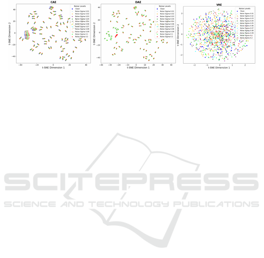
Figure 6: t-SNE plot of latent tensors for CAE, DAE, VAE.

tered around the origin. These observations reinforce

the behaviour that we observe in both the manifold

and Hilbert space analyses.

5.4 Discussion

In this subsection, we discuss the implications of the

observations from the results discussed earlier in this

section, focusing on their relevance to the denoising

application from the latent space perspective.

It is observed that the CAE and DAE have a latent

space which is a stratiﬁed manifold. While moving

within a stratum is smooth, transitioning across strata

is not so due to the dimensionality differences among

the strata. It is interesting to note that with increasing

noise, the manifold becomes a smooth SPD manifold

and moving from this higher rank manifold of SPD

matrices to the lower rank manifold of SPSD matrices

is easier as it only involves thresholding of the smaller

eigenvalues. This observation points to a possibility

of using both the autoencoders for denoising.

For VAEs, as outlined in (Lee and Lee, 2012, Ex-

ample 1.34), the Cartesian product of manifolds is

a smooth product manifold if each component man-

ifold is smooth. Since both SPD and SPSD (of ﬁxed

rank) are smooth manifolds, the latent space of the

VAE can be described as a smooth product manifold.

This smooth manifold structure may lead to far sim-

pler denoising algorithms than those with the CAEs

and DAEs. Our primary contribution lies in character-

izing the latent manifold as a product manifold of the

SPD/SPSD matrices, where the core distinction be-

tween smooth and non-smooth manifolds is rooted in

the structure of this product manifold. The CAE and

DAE form stratiﬁed product manifolds due to rank

variability of their respective SPSD matrices, leading

to discontinuities and non-smooth transitions across

strata. On the other hand, the VAE, with its uniform

rank structure, results in a smooth product manifold.

The Hilbert space analysis for the three autoen-

coders reveals the following structure. For the CAE

and DAE, the subspace representing noisy data ro-

tates away from that of clean data and has a lower di-

mension. Whereas, for the VAE, the noisy and clean

data points are transformed to latent space points that

can be mapped to the same Hilbert space. The t-SNE

plots also reﬂect these distinct structural differences

in latent spaces of the three autoencoders. The t-SNE

plot of VAE feature-points appear as a coherent ball

despite varying noise levels. Contrary to this, these

points are seen as elongated points in the t-SNE plot

for the CAE. The DAE, being midway between these

two, has more tightly clustered points.

All the three analysis methods provide strong and

concurring evidence for the smoothness of the latent

space of VAE and the non-smooth structure of latent

space of CAE and DAE.

6 CONCLUSION AND FUTURE

WORK

We characterize the latent spaces of different autoen-

coder models, speciﬁcally CAEs, DAEs and VAEs,

to gain an understanding of their respective smooth-

ness properties. For this, we explore the latent space

in two domains: the manifold space and the Hilbert

space. In the manifold space, with the help of a sim-

ple observation that the latent tensors lie on a prod-

uct manifold of the SPSD matrices, we observe the

variability in ranks of the SPSD matrices in the CAE

and DAE that result in a stratiﬁed structure, where

each stratum is smooth but the overall structure is

non-smooth due to discontinuities among strata. In

contrast, the VAE shows consistent ranks, forming

a smooth product manifold. In the Hilbert space,

varying dimensions and increasing principal angles

between clean and noisy subspaces in the CAE and

DAE suggest distinct subspaces for clean and noisy

data, while the VAE maintains the subspace with the

same dimensionality for both, with zero principal an-

gles. We also note a close relationship between sub-

VISAPP 2025 - 20th International Conference on Computer Vision Theory and Applications

space dimensionality and reconstruction performance

across models. These results are corroborated by the

t-SNE plots where signiﬁcant divergence is observed

between clean and noisy points in the CAE and DAE,

while such points for the VAE are tightly clustered

near the origin.

Much work remains to be done. We plan to extend

this analysis to other autoencoder variants and vali-

date the results with more datasets. Further, we also

plan to characterize the latent spaces of other genera-

tive models. As a constructive next step, we intend to

devise denoising and deblurring algorithms by lever-

aging the understanding of the manifold structure of

autoencoders, particularly VAEs.

REFERENCES

Abdelkader, M. F., Abd-Almageed, W., Srivastava, A., and

Chellappa, R. (2011). Silhouette-based gesture and

action recognition via modeling trajectories on Rie-

mannian shape manifolds. Computer Vision and Im-

age Understanding, 115(3):439–455.

Bengio, Y., Courville, A., and Vincent, P. (2013). Represen-

tation learning: A review and new perspectives. IEEE

Trans. on Pattern Analysis and Machine Intelligence,

35(8):1798–1828.

Berthelot, D., Raffel, C., Roy, A., and Goodfellow, I.

(2018). Understanding and improving interpola-

tion in autoencoders via an adversarial regularizer.

arXiv:1807.07543.

Bonnabel, S. and Sepulchre, R. (2010). Riemannian metric

and geometric mean for positive semideﬁnite matrices

of ﬁxed rank. SIAM Journal on Matrix Analysis and

Applications, 31(3):1055–1070.

Chadebec, C. and Allassonnière, S. (2022). A geomet-

ric perspective on variational autoencoders. Advances

in Neural Information Processing Systems, 35:19618–

19630.

Chen, N., Klushyn, A., Ferroni, F., Bayer, J., and Van

Der Smagt, P. (2020). Learning ﬂat latent manifolds

with VAEs. arXiv:2002.04881.

Connor, M., Canal, G., and Rozell, C. (Apr. 2021). Vari-

ational autoencoder with learned latent structure. In

Proc. AISTATS, Online.

Cristovao, P., Nakada, H., Tanimura, Y., and Asoh,

H. (2020). Generating in-between images through

learned latent space representation using variational

autoencoders. IEEE Access, 8:149456–149467.

Doersch, C. (2016). Tutorial on variational autoencoders.

arXiv:1606.05908.

Fefferman, C., Mitter, S., and Narayanan, H. (2016). Test-

ing the manifold hypothesis. Journal of the American

Mathematical Society, 29(4):983–1049.

Kingma, D. P. and Welling, M. (2013). Auto-encoding vari-

ational Bayes. arXiv:1312.6114.

Knyazev, A. V. and Zhu, P. (2012). Principal angles between

subspaces and their tangents. arXiv:1209.0523.

Lee, J. M. and Lee, J. M. (2012). Smooth manifolds.

Springer.

Leeb, F., Bauer, S., Besserve, M., and Schölkopf, B. (2022).

Exploring the latent space of autoencoders with in-

terventional assays. Advances in Neural Information

Processing Systems, 35:21562–21574.

Lui, Y. M. (2012). Human gesture recognition on prod-

uct manifolds. The Journal of Machine Learning Re-

search, 13(1):3297–3321.

Lui, Y. M., Beveridge, J. R., and Kirby, M. (Jun. 2010).

Action classiﬁcation on product manifolds. In Proc.

IEEE/CVF CVPR, San Francisco, CA.

Massart, E., Hendrickx, J. M., and Absil, P.-A. (Aug. 2019).

Curvature of the manifold of ﬁxed-rank positive-

semideﬁnite matrices endowed with the Bures–

Wasserstein metric. In Proc. Geometric Science of

Information Science (GSI), Toulouse, France.

Ng, A. et al. (2011). Sparse autoencoder. CS294A Lecture

notes, 72(2011):1–19.

Oring, A. (2021). Autoencoder image interpolation by

shaping the latent space. Master’s thesis, Reichman

University (Israel).

Rifai, S., Vincent, P., Muller, X., Glorot, X., and Bengio,

Y. (Jun. 2011). Contractive autoencoders: Explicit

invariance during feature extraction. In Proc. ICML,

Bellevue, WA.

Rodolà, E., Lähner, Z., Bronstein, A. M., Bronstein, M. M.,

and Solomon, J. (2019). Functional maps represen-

tation on product manifolds. In Computer Graphics

Forum. Wiley Online Library, pages 678–689.

Rumelhart, D. E., Hinton, G. E., and Williams, R. J. (1986).

Learning representations by back-propagating errors.

Nature, 323(6088):533–536.

Sharma, K. and Rameshan, R. (2021). Distance based ker-

nels for video tensors on product of Riemannian ma-

trix manifolds. Journal of Visual Communication and

Image Representation, 75:103045.

Sharma, K. and Rameshan, R. (May 2019). Linearized ker-

nel representation learning from video tensors by ex-

ploiting manifold geometry for gesture recognition. In

Proc. ICASSP, Brighton, UK.

Takatsu, A. (2011). Wasserstein geometry of Gaussian mea-

sures. Osaka J. Math, 48(4):1055–1026.

Van der Maaten, L. and Hinton, G. (2008). Visualizing data

using t-SNE. Journal of Machine Learning Research,

9(11).

Vincent, P., Larochelle, H., Bengio, Y., and Manzagol, P.-

A. (Jun. 2008). Extracting and composing robust fea-

tures with denoising autoencoders. In Proc. ICML,

Helsinki, Finland.

Zhai, J., Zhang, S., Chen, J., and He, Q. (Oct. 2018). Au-

toencoder and its various variants. In Proc. IEEE

SMC, Miyazaki, Japan.

Zhang, K., Lan, L., Wang, Z., and Moerchen, F. (Apr.

2012). Scaling up kernel SVM on limited resources:

A low-rank linearization approach. In Proc. AISTATS,

La Palma, Canary Islands.

Latent Space Characterization of Autoencoder Variants