Sequential Counter Encoding for Staircase At-Most-One Constraints

Hieu Xuan Truong, Tuyen Van Kieu and Khanh Van To

VNU University of Engineering and Technology, Vietnam

{truongxuanhieu11, tuyenkv, khanhtv}@vnu.edu.vn

Keywords:

CNF Encoding, Sequential Counter Encoding, Sequence Constraints, Anti-Bandwidth.

Abstract:

This paper presents a new SAT encoding to represent Staircase At-Most-One (SCAMO) constraints by

combining similar sub-formulae between At-Most-One (AMO) constraints within constructing blocks. The

SCAMO constraints exhibit a staircase shape due to the structural similarity between consecutive AMO con-

straints. The proposed method utilizes Sequential Counter (SC) encoding to represent each block in a staircase

form, taking advantage of connecting the constraint representation for two consecutive blocks. Compared to

the existing SCAMO representation based on Binary Decision Diagrams (BDD), our method requires fewer

variables and clauses, resulting in improved solving time for SCAMO. Experimental results on real-world

problems, such as Anti-bandwidth problems, demonstrate that the SC encoding representation method for

SCAMO consistently outperforms alternative methods.

1 INTRODUCTION

Sequence constraints are a common type of con-

straint appearing in many combinatorial problems,

such as Car Sequencing, Nurse Rostering, and Em-

ployee Scheduling or Crew Rostering. For exam-

ple, in the Car Sequencing problem (Artigues et al.,

2014) (Siala, 2015), a sequence constraint limits the

at-most number of cars in a sequence that can be as-

sembled with a particular option. In the Nurse Ros-

tering problem (Ceschia et al., 2015) (Kletzander and

Musliu, 2020), a constraint might limit nurses to work

a maximum of 3-night shifts in 7 consecutive work-

ing days. Similarly, the Employee Scheduling prob-

lem (Nieuwenhuis et al., 2021) has a fairness con-

straint to balance morning and afternoon shifts. Se-

quence constraints restrict the number of occurrences

of certain values in a sequence of k variables, denoted

as AmongSeq (Bessiere et al., 2007) and AtMostSeq

(Artigues et al., 2014).

Sequence constraint is also in the anti-bandwidth

problem (Sinnl, 2021), applied for many applications

in scheduling (Leung et al., 1984), radio frequency

assignment (Hale, 1980), obnoxious facility location

(Cappanera, 1999) and map coloring (Hu et al., 2010).

SAT solving is used in many real-life applications

because SAT solvers have signiﬁcantly improved in

strength. When applying SAT encoding to combi-

natorial problems, a large number of clauses are of-

ten generated. To address this issue, various encod-

ing techniques have been proposed to reduce the sig-

niﬁcant number of clauses (Haberlandt et al., 2023)

(Vasconcellos-Gaete et al., 2020).

In our paper, we focus on addressing the At-

Most-One (AMO) sequence constraints, which means

that in any k consecutive elements, there is at most

1 element with the value TRUE. This constraint is

called the Staircase At Most One (SCAMO) con-

straint (Fazekas et al., 2020). The paper presents a

new SAT encoding for SCAMO by leveraging similar

sub-formulae to encode for a set of AMOs instead of

encoding each AMO separately. Our new encoding is

based on the sequential counter encoding (SC) (Sinz,

2005), instead of applying BDD as in (Fazekas et al.,

2020). The set of AMO constraints is divided into

blocks that share similar sub-formulae among AMO

constraints and then SC encoding is applied to repre-

sent a block and its neighboring blocks. This is done

to reduce the number of clauses required when encod-

ing each AMO constraint separately.

The key contributions of our research are as fol-

lows:

• We propose an efﬁcient SAT encoding for

SCAMO constraints, which signiﬁcantly reduces

the number of variables and clauses compared to

using BDD and other encodings to represent each

AMO separately.

• We propose an efﬁcient SAT encoding to solve the

anti-bandwidth problems.

164

Truong, H. X., Van Kieu, T. and Van To, K.

Sequential Counter Encoding for Staircase At-Most-One Constraints.

DOI: 10.5220/0013124600003890

Paper published under CC license (CC BY-NC-ND 4.0)

In Proceedings of the 17th International Conference on Agents and Artiﬁcial Intelligence (ICAART 2025) - Volume 2, pages 164-175

ISBN: 978-989-758-737-5; ISSN: 2184-433X

The paper is organized as follows: Section 1 in-

troduces the research problem and summarizes the

new contributions of this study. Section 2 covers the

fundamentals of SCAMO constraints and encodings

using Binary Decision Diagrams (BDD). Section 3

presents our approach to representing SCAMO us-

ing SC. Section 4 discusses the Antibandwidth prob-

lem and its reduction to propositional logic formu-

las. Section 5 details the experiments comparing our

new SCAMO encoding with BDD, as well as the en-

coding techniques for each AMO constraint individ-

ually, including the experimental results for the Anti-

bandwidth problem. Finally, Section 6 concludes the

paper.

2 STAIRCASE AT-MOST-ONE

CONSTRAINTS

2.1 SCAMO Deﬁnition

The Staircase At-Most-One (SCAMO) constraint, as

discussed in (Fazekas et al., 2020), is a specialized

variant of the At-Most-One (AMO) constraint. The

SCAMO constraint set is created when a series of

AMO constraints share overlapping variables across

consecutive constraints, forming a “staircase” struc-

ture. This arrangement allows for the reuse of inter-

mediate results among these consecutive constraints,

thereby reducing the number of variables and clauses

required for encoding.

Deﬁnition 1. Given a sequence of n Boolean vari-

ables Ω = {x

, x

, ..., x

} and a number w st. 1 < w ≤

n, a SCAMO with a width of w is formulated as fol-

lows:

SCAMO(Ω, w) =

n−w

i=0

(

∑

i+w

j=i+1

≤ 1)

Example 1. Given a sequence of 10 Boolean vari-

ables Ω = {x

, x

, ..., x

}, the SCAMO constraints of

the 4-width staircase can be illustrated as follows:

+ x

≤ 1∧

+ x

≤ 1∧

+ x

≤ 1∧

+ x

≤ 1∧

+ x

≤ 1∧

+ x

≤ 1∧

+ x

≤ 1

The SCAMO constraint, as deﬁned in Deﬁnition

1 and illustrated in Example 1, can be decomposed

into a set of overlapping AMO constraints that slide

over the sequence of variables. The key feature of

this “staircase” structure is the overlap between con-

secutive constraints. For instance, in Example 1, the

ﬁrst and second constraints both include the variables

, x

, and the second and third constraints share

the variables x

, x

. This overlap allows reuse of

previous computation to evaluate the ﬁrst AMO con-

straint as x

+ (x

+ x

), which can just consider

the sub-expression (x

+ x

) together with x

evaluate the second AMO constraint. In general, each

successive constraint shares a sum over w −1 vari-

ables with both the previous constraint and the next

constraint, allowing partial reuse of sub-expressions

across constraints, as shown in Deﬁnition 1.

2.2 Decomposition of SCAMO

Efﬁcient encoding of SCAMO constraints necessi-

tates their decomposition into smaller, reusable sub-

constraints. This decomposition strategy minimizes

the number of variables and clauses required and

leverages the inherent overlapping nature of SCAMO

constraints to enhance computational efﬁciency. We

illustrate the decomposition of SCAMO constraints in

Figure 1.

Proposition 1. The constraint x

+ x

+ . . . + x

≤ 1

holds iff for all 1 ≤i < n :

+ . . . + x

≤ 1) ∧(x

i+1

+ . . . + x

≤ 1)∧

+ . . . + x

≤ 0 ∨x

i+1

+ . . . + x

≤ 0)

Encoding SCAMO constraints requires break-

ing down the larger constraints into smaller sub-

constraints that can be reused across consecutive win-

dows of variables. To begin the decomposition, we

ﬁrst partition the sequence of Boolean variables Ω =

⟨

, x

, . . . , x

⟩

into M =





consecutive “windows”,

where each window contains w variables, except

possibly the last window, which may contain fewer

variables if n mod w ̸= 0. Formally, each window

contains the variables ω

⟨

, x

, . . . , x

⟩

, ω

⟨

w+1

, x

w+2

, . . . , x

⟩

, etc.

The encoding process begins with the construction

of individual constraints for each AMO constraint de-

rived from the SCAMO decomposition. Each con-

straint accurately captures the exclusivity condition of

its respective AMO constraint. However, to maintain

the staircase structure, it is imperative to ensure con-

sistency across overlapping variables in consecutive

AMO constraints. This is achieved by introducing At-

Most-Zero (AMZ) constraints, as shown in Proposi-

tion 1. The AMZ constraints ensure that shared vari-

ables do not violate the exclusivity conditions when

transitioning between blocks. Speciﬁcally, the AMZ

constraints (x

+ . . . + x

≤ 0 ∨x

i+1

+ . . . + x

≤ 0)

in Proposition 1 guarantee that at least one of the

two sub-expressions must be zero. This, combined

with the individual AMO constraints on each sub-

expression, maintains the overall at-most-one prop-

erty across the entire set of variables. Applying this

Sequential Counter Encoding for Staircase At-Most-One Constraints

165

+ (x

)))) ≤ 1

+ (x

))) + (x

) ≤ 1

+ (x

)) + ((x

) + x

) ≤ 1

) + (((x

) + x

) ≤ 1

((((x

) + x

) ≤ 1

+ (x

)))) ≤ 1

+ (x

)))) ≤ 1

+ (x

)))) ≤ 1

)

Figure 1: Decomposition of SCAMO.

+ x

≤ 1

+ x

≤ 1 x

+ x

≤ 1

+ x

≤ 0 x

+ x

≤ 0

+ x

≤ 0

⊤

⊥

+ x

≤ 1

+ x

≤ 1

+ x

≤ 1

+ x

≤ 0 x

+ x

≤ 0

+ x

≤ 0 x

≤ 0

⊥

⊤

¬x

Figure 2: Forward and backward BDDs for SCAMO constraints (Fazekas et al., 2020).

proposition to the SCAMO constraint illustrated in

Figure 1, the constraint x

+ x

≤ 1 can be

decomposed into:

≤ 1) ∧(x

+ x

≤ 1)∧

≤ 0 ∨x

+ x

≤ 0)

2.3 BDD Encoding for SCAMO

To encode AMO and AMZ constraints, we use BDD

encoding (Bryant, 1986), (Akers, 1978) to represent

the constraints in a compact form. The BDD en-

coding consists of two parts: forward and backward

BDDs for each window of variables. Forward BDD

(ω

) is constructed using a right-associative variable

ordering, where variables are ordered from x

to x

. It

captures the AMO and AMZ constraints for the win-

dow, ensuring that At-Most-One variable can be set

to true. Backward BDD (ω

) uses a left-associative

ordering, starting from the last variable x

and pro-

ceeding backward to x

. Figure 2 illustrates two

BDDs of ω

, ω

with ordering x

≺ x

and

≺ x

respectively in Example 1.

To maintain consistency across overlapping AMO

constraints in consecutive windows, the forward BDD

of one window is bonded to the backward BDD of

the subsequent window. Speciﬁcally, for each pair

of consecutive windows ω

and ω

i+1

, the j

layer of

is connected to the (w − j + 2)

layer of ω

i+1

where 2 ≤ j ≤ w. This bonding is enforced through

binary clauses that synchronize the sub-constraints of

overlapping variables, ensuring that shared variables

adhere to the SCAMO constraints without redundant

encodings. On layers ω

-BDD and ω

-BDD, we have

following sub-formulae:

+ x

≤ 1)

∧(x

+ x

≤ 1) ∧(x

≤ 1)

∧(x

+ x

≤ 0 ∨x

≤ 0)

∧(x

+ x

≤ 1) ∧(x

+ x

≤ 1)

∧((x

+ x

≤ 0) ∨(x

+ x

≤ 0))

∧(x

≤ 1) ∧(x

+ x

≤ 1)

∧((x

≤ 0) ∨(x

+ x

≤ 0))

ICAART 2025 - 17th International Conference on Agents and Artiﬁcial Intelligence

166

Duplex encoding (Fazekas et al., 2020) lever-

ages BDDs to systematically decompose and en-

code SCAMO constraints, and reduces the number

of clauses compared to naive encoding by reusing

sub-constraints. It introduces additional complexity

in both clause generation and memory usage, lead-

ing to increased clause generation (N(3(w − 2) +

2(w −1) −1) clauses), especially in larger problem

instances (in the worst case it is O





). The need

for auxiliary variables to bond BDDs across windows

adds to the memory overhead (N(2w − 3)). Each

window requires multiple variables for both AMO

and AMZ constraints, which may cause inefﬁciencies

when scaling to larger datasets or higher dimensions.

3 THE SC ENCODING FOR

SCAMO CONSTRAINTS

In this section, we will introduce our method for en-

coding SCAMO, called SCL (Sequential Counter en-

coding for Ladder constraints). Our approach takes

advantage of the reusable potential of decomposed

constraints. First, we break down the large SCAMO

into smaller blocks based on related sub-expressions.

These related sub-expressions can then be encoded

into a single Sequential Counter (SC), which gener-

ates some auxiliary register bits. Finally, we connect

these auxiliary bits to reformulate the original con-

straints of the SCAMO.

3.1 SCL Encoding for SCAMO

Given a SCAMO set of width w over n variables,

let Ω = {x

, x

, . . . , x

}, we divide Ω into M =





subsets, denoted as {ω

, . . . , ω

}. Each subset con-

tains up to w unique variables, such that ω

i,1

, . . . , x

i,w

}. For each subset ω

, we create two SC

blocks that represent the constraint (x

i,1

+ . . . + x

i,w

≤

1) by using different variable orderings: a left order-

ing starting from x

i,1

to x

i,w

and a right ordering start-

ing from x

i,w

to x

i,1

. The sub-expressions obtained

from the SC construction of adjacent blocks can then

be combined to reconstruct the AMO constraints of

the original SCAMO.

As illustrated in Figure 1, the set of variables in

the example SCAMO is divided into three subsets:

= {x

, x

}, ω

= {x

, x

}, and ω

, x

}. Constructing ω

using SC with right vari-

able ordering yields a block of four sub-expressions:

1,1

= {x

}, R

1,2

= {x

}, R

1,3

= {x

}and

1,4

= {x

+ x

}. Similarly, constructing ω

using the same method but in reverse order produces

another block of four sub-expressions: R

2,1

= {x

2,2

= {x

+ x

}, R

2,3

= {x

+ x

}, and R

2,4

}. Combining R

1,3

and R

2,1

results in

the expression {x

+ x

}. Meanwhile, com-

bining R

1,2

and R

2,2

yields {x

+ x

}, and so

on for other combinations.

We observe that when two blocks represent the

same set of variables but are ordered differently, it is

sufﬁcient to use only one of these blocks to satisfy

the AMO constraint. We refer to the block that satis-

ﬁes the AMO constraint as the AMO block, while the

other block is called the AMZ block.

Note that the ﬁrst and the last subsets are the spe-

cial cases. They are adjacent to only one subset, ei-

ther on the left or the right side, unlike the other

subsets, which are adjacent to two subsets on both

sides. Therefore, their construction consists of only

one block with the AMO constraint, i.e., the AMO

block.

Let R

i, j

represent the register bit that indicates the

sum of the ﬁrst j variables. Let x

i, j

denote the j

vari-

able of block B

according to the variable ordering.

The relationship for R

i, j

is deﬁned as follows:

i, j

is true if and only if

∑

′

i, j

′

= 1,

which means that exactly one of the ﬁrst j variables in

block B

is true. Conversely,

i, j

is false if and only if

∑

′

i, j

′

≤ 0,

indicating that all of the ﬁrst j variables in block B

are false.

AMO and AMZ blocks are encoded by the follow-

ing four formulas:

(1)

j=2

i, j

→ R

i, j

(2)

j=2

i, j−1

→ R

i, j

(3)

j=2

¬x

i, j

∧¬R

i, j−1

→ ¬R

i, j

(4)

j=2

i, j

→ ¬R

i, j−1

Formula (1) sets the register bits R

i, j

to true when

i, j

is true. Formula (2) sets R

i, j

to true if the previous

i, j−1

is true. Formula (3) sets R

i, j

to false

when all the j variables are false. Finally, we include

formula (4) to ensure that at most one variable can be

true.

For example, we indexed four blocks derived from

the decomposition of the SCAMO as illustrated in

Figure 1. The corresponding register bits of their sub-

expressions are shown in Figure 3. Block B

repre-

sents the ﬁrst subset and must therefore be classiﬁed

as an AMO block. Its construction utilizes all four

formulas as follows:

Sequential Counter Encoding for Staircase At-Most-One Constraints

167

+ (x

)))) ≡ R

1,4

+ (x

))) ≡ R

1,3

+ (x

)) ≡ R

1,2

) ≡ R

1,1

) ≡ R

2,1

((x

) + x

) ≡ R

2,2

(((x

) + x

) ≡ R

2,3

((((x

) + x

) ≡ R

2,4

+ (x

)))) ≡ R

3,4

+ (x

))) ≡ R

3,3

+ (x

)) ≡ R

3,2

) ≡ R

3,1

≡ R

4,1

(((x

)) + x

) ≡ R

4,2

Figure 3: Register bits constructing of SC blocks.

(1)

j=2

⇐⇒

1,2

→ R

1,2

1,3

→ R

1,3

1, j

→ R

1, j

1,4

→ R

1,4

(2)

j=2

⇐⇒

1,1

→ R

1,2

→ R

1,3

1, j−1

→ R

1, j

1,3

→ R

1,4

(3)

j=2

⇐⇒

¬x

1,2

∧¬R

1,1

→ ¬R

1,2

¬x

1,3

∧¬R

1,2

→ ¬R

1,3

¬x

1, j

∧¬R

1, j−1

→ ¬R

1, j

¬x

1,4

∧¬R

1,3

→ ¬R

1,4

(4)

j=2

⇐⇒

1,2

→ ¬R

1,1

1,3

→ ¬R

1,2

1, j

→ ¬R

1, j−1

1,4

→ ¬R

1,3

According to the variable ordering of block B

we have x

1,1

≡ x

, x

1,2

≡ x

, x

1,3

≡ x

, x

1,4

≡ x

, and

≡ R

1,1

. As a result, the constraints above are now

equivalent to:

1,2

→ R

1,2

⇐⇒

→ R

1,2

1,3

→ R

1,3

→ R

1,3

1,4

→ R

1,4

→ R

1,4

1,1

→ R

1,2

⇐⇒

→ R

1,2

→ R

1,3

1,2

→ R

1,3

→ R

1,4

1,3

→ R

1,4

¬x

1,2

∧¬R

1,1

→ ¬R

1,2

⇐⇒

¬x

∧¬x

→ ¬R

1,2

¬x

1,3

∧¬R

1,2

→ ¬R

1,3

¬x

∧¬R

1,2

→ ¬R

1,3

¬x

1,4

∧¬R

1,3

→ ¬R

1,4

¬x

∧¬R

1,3

→ ¬R

1,4

1,2

→ ¬R

1,1

⇐⇒

→ ¬x

1,3

→ ¬R

1,2

→ ¬R

1,2

1,4

→ ¬R

1,3

→ ¬R

1,3

Let block B

be an AMO block from the second

subset. The construction of the block B

is as follows:

→ R

2,2

¬x

∧¬x

→ ¬R

2,2

→ R

2,3

¬x

∧¬R

2,2

→ ¬R

2,3

→ R

2,4

¬x

∧¬R

2,3

→ ¬R

2,4

→ R

2,2

→ ¬x

2,2

→ R

2,3

→ ¬R

2,2

2,3

→ R

2,4

→ ¬R

2,3

The block B

also represents the second subset,

just as block B

does. Since block B

is an AMO

block, block B

is designated as an AMZ block and

is constructed without applying formula (4):

→ R

3,2

¬x

∧¬x

→ ¬R

3,2

→ R

3,3

¬x

∧¬R

3,2

→ ¬R

3,3

→ R

3,4

¬x

∧¬R

3,3

→ ¬R

3,4

→ R

3,2

→ R

3,3

→ R

3,4

The block B

represents the ﬁnal subset and can

be constructed using the same method as the B

and

blocks. The important point is that B

is an in-

complete block; its width is only 2. Therefore, rather

than creating a wide SC of length w, we will create an

SC that matches the actual width of the B

block by

implementing the following constraints:

→ R

4,2

¬x

∧¬x

→ ¬R

4,2

→ R

4,2

→ ¬x

After breaking down into SC blocks, we need

to connect these blocks to reformulate the original

SCAMO. In this process, we connect each block

from every subset to the corresponding block of the

neighboring subsets.

The connection between blocks B

and B

is in-

tended to reformulate the following ﬁve AMO con-

straints:

+ x

≤ 1)∧

+ x

≤ 1)∧

+ x

≤ 1)∧

+ x

≤ 1)∧

+ x

≤ 1)

Proposition 1 is applied to decompose these ﬁve

constraints into:

+ x

≤ 1)∧

+ x

≤ 1) ∧(x

+ x

≤ 0 ∨x

≤ 0)∧

+ x

≤ 1) ∧(x

+ x

≤ 1) ∧(x

+ x

≤ 0 ∨x

+ x

≤ 0)∧

≤ 1) ∧(x

+ x

≤ 1) ∧(x

≤ 0 ∨x

+ x

≤ 0)∧

+ x

≤ 1)

The resulting AMZ constraints can then be re-

placed with the corresponding register bits as follows:

ICAART 2025 - 17th International Conference on Agents and Artiﬁcial Intelligence

168

Table 1: Size of SAT encoding for a SCAMO constraint over n variables with width w.

Encoding Auxiliary variables Clauses Complexity

Naive 0

N(w −1)w O(n

)

Reduced 0

(w −1)w + (N −1)(w −1) O(n

)

Seq N(w −2) N(3(w −2) + 1) O(n

)

BDD N(2w −3) N(3(w −2) + 2(w −1) −1) O(n

)

2-product N(2

√

w + O

√

w) N(2w + 4

√

w + O

√

w) O(n

)

Duplex 4Mw −4M 13Mw −14M −3w + 2 O(n)

SCL 2Mw −3M −2w + 4 8Mw −8M −7w + 7 O(n)

+ x

≤ 1)∧

+ x

≤ 1) ∧(x

≤ 1) ∧(¬R

1,3

∨¬x

)∧

+ x

≤ 1) ∧(x

+ x

≤ 1) ∧(¬R

1,2

∨¬R

2,2

)∧

≤ 1) ∧(x

+ x

≤ 1) ∧(¬x

∨¬R

2,3

)∧

+ x

≤ 1)

Likewise, the connection between blocks B

and

is encoded by:

+ x

≤ 1)∧

+ x

≤ 1)∧

+ x

≤ 1)

≡

+ x

≤ 1)∧

+ x

≤ 1) ∧(x

≤ 1) ∧(¬R

3,3

∨¬x

)∧

+ x

≤ 1) ∧(x

+ x

≤ 1) ∧(¬R

3,2

∨¬R

4,2

)

All in all, given two blocks that represent two

consecutive windows of width w {x

, . . . , x

i+w

} and

i+w+1

, . . . , x

i+w+w

}. Connecting these two blocks re-

quires w −1 clauses:

∑

j=2

(

∑

i+w

k=i+ j

≤ 0 ∨

∑

i+w+ j−1

′

=i+w+1

′

≤ 0)

3.2 Comparison of SCAMO Encodings

In this section, we compare our proposed SCL encod-

ing with Duplex (Fazekas et al., 2020) and several en-

codings for each AMO constraint, including Pairwise,

Sequential Counter (Sinz, 2005), BDD (Ab

ıo et al.,

2012), and 2-Product (Chen, 2010).

Table 1 presents the results concerning the number

of new variables and clauses generated for each en-

coding, both from the study by (Fazekas et al., 2020)

and our SCL encoding. The Naive method utilized

Pairwise encoding, while the Reduced method elimi-

nated duplicate binary clauses in the pairwise encod-

ing process. Note that in Table 1, N = (n −w) + 1 and

M =





The Duplex encoding encodes each window sepa-

rately by creating two BDDs, each containing 2(w +

1) nodes. After constructing these diagrams, the lay-

ers of the neighboring BDDs are connected, result-

ing in M −1 bond clauses. According to the esti-

mation in (Fazekas et al., 2020), Duplex encoding re-

quires approximately 13Mw −14M −3w + 2 clauses

and 4Mw −4M auxiliary variables.

When comparing the construction of two BDDs

used in Duplex encoding with our SCL encoding, we

ﬁnd that SCL requires fewer variables and clauses. To

simplify the calculation, let’s assume that each block

has the same size, although most of the time the last

block is smaller. For the ﬁrst and last subsets, SCL

creates one AMO block, while for the remaining (M-

2) subsets, SCL creates one AMO block and one AMZ

block each. This results in a total of M AMO blocks

and M −2 AMZ blocks. Additionally, M + M −2 =

2M −2 blocks require M −1 connections. In con-

clusion, the number of clauses in SCL encoding is:

AMO-block-clauses ≤ M(4(w −1))

= 4Mw −4M

AMZ-block-clauses ≤ (M −2)(3(w −1))

= 3Mw −3M −6w + 6

Connect-clauses ≤ (M −1)(w −1)

= Mw −M −w + 1

Total-clauses = AMO-block-clauses +

AMZ-block-clauses +

Connect-clauses +

≤ 8Mw −8M −7w + 7

The total number of auxiliary variables in our en-

coding is at most (w −1) + (M −2)((w −1) + (w −

2) + (w −1)) = 2Mw −3M −2w + 4. In this expres-

sion, the ﬁrst and last (w −1) variables are used to

encode the AMO block of the ﬁrst and last subsets.

The remaining (M −2)((w −1) + (w −2)) variables

are used to encode the (M −2) subsets between the

ﬁrst and last subsets, with each subset using (w −1)

variables for the AMO block and (w−2) variables for

the AMZ block. The AMZ blocks require one variable

less than the AMO blocks because the highest regis-

ter bits of both blocks are the same, allowing AMZ

blocks to reuse them from the AMO blocks instead of

creating new ones. For example, the register bit R

2,4

block B

and the register bit R

3,4

of block B

in Figure

3 both represent {x

}, hence R

2,4

≡R

3,4

Table 1 shows the number of auxiliary variables,

the number of clauses, and the complexity of differ-

ent SAT encodings in the SCAMO constraint set of n-

variable with AMO constraints of width w. The com-

plexity of each approach is calculated based on the

number of clauses in the worst case (i.e., w is approx-

imately

Sequential Counter Encoding for Staircase At-Most-One Constraints

169

Figure 4: Comparison of the number of clauses of a

SCAMO with parameters set to n = 1000 and w ∈(1, 1000).

The theoretical calculations provided above show

that our proposed encoding demonstrates superior

performance in terms of the number of clauses. It has

linear complexity and uses just over half the number

of variables compared to the Duplex encoding, which

also has linear complexity. Importantly, our SCL en-

coding requires fewer auxiliary variables than the Se-

quential counter, BDD, 2-product, and even Duplex

encodings. The Naive and Reduced encodings are the

only ones that do not use any auxiliary variables; how-

ever, their complexities of O(n

) and O(n

) cannot be

compared to our complexity of O(n).

Figures 4 and 5 illustrate the number of clauses

and auxiliary variables needed to encode a set of

SCAMO constraints with n = 1000 and w ∈ (1, 1000)

for various SAT encodings, based on calculations

from Table 1.

4 ANTI-BANDWIDTH PROBLEM

We apply our proposed method to the anti-bandwidth

problem (ABP) (Sinnl, 2021), which is an NP-hard

problem with applications in various scheduling sce-

narios, including radio frequency assignment, obnox-

ious facility location, and map coloring.

4.1 Problem Deﬁnition

Let G = (V, E) be a graph where V is the set of vertices

and E is the set of edges. Let n = |V| be the number

of vertices, and m = |E| be the number of edges. A la-

beling f of the vertices is a bijection V → {1, ..., n}

such that each vertex i ∈ V receives a unique label

f(i) ∈ {1, ..., n}.

Given graph G and labeling f, AB

(i) is the mini-

mum bandwidth of vertex i ∈V and the labeling f:

(i) = min{|f (i) − f (i

′

)| : {i, i

′

} ∈ E}

Figure 5: Comparison of the number of auxiliary vari-

ables of a SCAMO with parameters set to n = 1000 and

w ∈(1, 1000).

The bandwidth of G is the minimal value among

the AB

(i) values:

(G) = min{AB

(i) : i ∈V }

Let F(G) denote all labels of G. The anti-

bandwidth problem aims at ﬁnding a labeling f

∗

that

maximizes the bandwidth of G. The corresponding

value AB

∗

(G) is called anti-bandwidth AB(G) of G,

i.e.,

AB(G) = max

f ∈F

(G)

4.2 Constraint Representation

(Duarte et al., 2011) introduced a mixed-integer

programming (MIP) approach to provide a solution

to ABP. Then, based on the MIP approach, (Sinnl,

2021) presented an iterative formulation, which is

a feasibility problem, to answer the question “Does

there exist a solution with AB(G) ≥ k + 1?”. This

iterative approach can be stated as follows:

Let boolean variables x

take the value true i f f

vertex i gets labels l, i.e. f

= l. To make sure that

every vertex gets a unique labeling, the following set

of constraints (V ERT ICES) and (LABELS) are used:

∑

i∈V

= 1 ∀l ∈ {1, . . . ,

} (V ERT ICES)

∑

l∈{1,...,

}

= 1 ∀i ∈V (LABELS)

If k is a feasible bandwidth of the ABP, the con-

straint (OBJ −k), which makes sure that for each edge

{i, i

′

} ∈ E, the difference between the labeling of ver-

tex i and i

′

must not be lower than or equal to k, must

be satisﬁed; otherwise, it is unsatisﬁed:

∑

2+k

′

+ x

′

) ≤ 1 ∀{i, i

′

} ∈ E (OBJ −k)

∀1 ≤ l

≤

−k

ICAART 2025 - 17th International Conference on Agents and Artiﬁcial Intelligence

170

This iterative approach ﬁrstly assigns k ← 1 then

solves the set of three constraints above. After that,

it continues to increase k by one and restart the solv-

ing process until we obtain an unsatisﬁed result. The

value of k when the solution process yields the value

unsatis f iability is the AB(G) of ABP.

For each edge in E, there should be an OBJ −k

constraint to ensure that the difference between the

two vertices of that edge is at least k. It means encod-

ing all the edges in E results in

different SCAMOs.

In order to reduce the number of SCAMOs, (Fazekas

et al., 2020) uses Proposition 1 to decompose (OBJ −

k) constraints into:

∑

2+k

′

+ x

′

) ≤ 1

Prop. 1

≡

∑

2+k

′

≤ 1 ∧

∑

2+k

′

≤ 1∧

(

∑

2+k

′

≤ 0 ∨

∑

2+k

′

≤ 0)

This decomposition breaks a SCAMO of an edge

into two SCAMOs of a single vertex. Since the num-

ber of edges

is much more than the number of

vertices

in most of the graphs, the number of

SCAMOs obtained from this decomposition after ter-

minating all duplicates is lower than from the origi-

nal OBJ −k constraints. Then, the two SCAMOs are

reconnected using a dis junction of some AMZ con-

straints of width k + 1, which can be formulated by

combining our constructed AMZ sub-expressions in

SCAMOs, as outlined in Proposition 2:

Proposition 2. A constraint x

+ x

+ . . . + x

≤ 0

holds iff for all 1 ≤ i < n :

+ . . . + x

≤ 0) ∧(x

i+1

+ . . . + x

≤ 0)

Let the SCAMO in Figure 1 be the SCAMO of a

single vertex got from decomposing a SCAMO of an

edge. The connect dis junction now contains all the

constraints of the SCAMO in Figure 1 but in AMZ

form, such as (x

+ x

≤ 0). Proposition 2

then breaks the constraint (x

+ x

≤ 0) into

+ x

≤ 0) ∧(x

≤ 0), which is equivalent to

¬R

1,3

∧¬R

2,1

(see Figure 3).

Take note that the (LABELS) constraint can be

formulated by merging subsets in corresponding

SCAMO, so instead of creating AMO constraints for

all variables, we focus on creating AMO constraints

for the subsets only. Because every subset also is

an AMO constraint and already constructed in the

(OBJ-k) constraint, this approach not only yields the

same result but also takes advantage of reusing subset

constructions. For example, in the Figure 1, instead

of creating the AMO constraint of all the 10 variables,

we only need to create the AMO constraint of 3

subsets {x

, x

}, {x

, x

} and {x

, x

In addition, we can see that for every labeling f

of the n-vertex graph, there exists a corresponding re-

versed labeling f

′

where f

′

= n + 1 − f . Since f

′

a linear transformation of f , it ensures that for each

value in f , there is exactly one corresponding value

in f

′

. This means that if f satisﬁes the conditions

of (V ERT ICES) and (LABELS) then f

′

also satisﬁes

these conditions. Furthermore, f

′

maintains the same

bandwidth as f :

′

(i) − f

′

)

(n + 1 − f (i)) −(n + 1 − f (i

′

))

f (i

′

) − f (i)

Based on this observation, we apply the symme-

try breaking technique (Gent et al., 2006) to reduce

the search space. In our implementation of ABP, we

employ symmetry breaking at one selected node us-

ing two different conﬁgurations: the ﬁrst node and the

highest-degree node.

5 EXPERIMENTAL EVALUATION

5.1 Experimental Setup

We implemented two frameworks to compare state-

of-the-art methods with our proposed encoding, SCL.

The ﬁrst framework focuses on the SCAMO, while

the second focuses on the ABP.

In the ﬁrst framework

, we compare SCL along-

side ﬁve other SAT encodings: Naive, Reduced, Se-

quential counter, 2-product (Product), and Duplex, as

detailed in Section 3.2. These methods were applied

to a SCAMO with parameters set to n = 1000 and w

varying between 1 and 1000.

In the second framework

, in addition to our pro-

posed encoding and the other SAT encodings from

the ﬁrst framework, we also included several Con-

straint Programming (CP) and Mixed Integer Pro-

gramming (MIP) approaches. We benchmarked our

experiments using 24 matrices from the Harwell-

Boeing Sparse Matrix Collection (Rodriguez-Tello

et al., 2015), which consists of 12 relatively small

to medium-sized graphs and 12 signiﬁcantly larger

graphs. These matrices were tested on a cluster in

Google Cloud Platform

with conﬁgurations of ma-

chine type e2-highmem-8 (8 vCPUs, 4 cores, 64GB

memory) and Debian GNU/Linux 12 operating sys-

tem. For selected SAT solver, we used version 1.2.1

of the CaDiCal solver (Biere, 2019).

Table 2 presents information on 24 matrices, in-

cluding their names, the number of vertices |V |, and

https://github.com/TruongXuanHieu-H/

StaircaseEncoderSCL.git

https://github.com/TruongXuanHieu-H/

AntiBandwidthSCL.git

https://console.cloud.google.com/compute

Sequential Counter Encoding for Staircase At-Most-One Constraints

171

Table 2: Harwell-Boeing Sparse Matrix benchmark.

Instance

| |

LB UB

A-pores 1 30 103 6 8

B-ibm32 32 90 9 9

C-bcspwr01 39 46 16 17

D-bcsstk01 48 176 8 9

E-bcspwr02 49 59 21 22

F-curtis54 54 124 12 13

G-will57 57 127 12 14

H-impcol b 59 281 8 8

I-ash85 85 219 19 27

J-nos4 100 247 32 40

K-dwt 234 117 162 46 58

L-bcspwr03 118 179 39 39

M-bcsstk06 420 3720 28 72

N-bcsstk07 420 3720 28 72

O-impcol d 425 1267 91 173

P-can 445 445 1682 78 120

Q-494 bus 494 586 219 246

R-dwt 503 503 2762 46 71

S-sherman4 546 1341 256 272

T-dwt 592 592 2256 103 150

U-662 bus 662 906 219 220

V-nos6 675 1290 326 337

W-685 bus 685 1282 136 136

X-can 715 715 2975 112 142

the number of edges |E|. The corresponding lower

and upper bounds (LB and UB) are provided in

(Fazekas et al., 2020).

5.2 Evaluation for the SCAMO

We have evaluated the performance in terms of solv-

ing time for the given SCAMO with n = 1000 vari-

ables, where the width w was adjusted from 5 to 995

(i.e., 5, 10, 15, . . . , 995), as shown in Figure 6. Among

the three best encodings, SCL emerged as the most

effective, surpassing Duplex, which was previously

found to be the efﬁcient encoding. A detailed com-

parison of all implemented encodings can be found

in Figure 9 in the Appendix. Overall, the results in-

dicate that, in most cases, the SCL encoding signiﬁ-

cantly outperforms all other SAT encodings in terms

of time efﬁciency. Additionally, the effectiveness of

the generated clauses and the required auxiliary vari-

ables for SCL are discussed earlier in Figure 4 and 5.

5.3 Evaluation for the ABP

In the second framework, we implemented our ap-

proach along with four SAT encodings: Product, Re-

duced, Sequential counter, and Duplex. We followed

the same process throughout. Initially, we consider

Figure 6: Comparison of solving time for three best encod-

ings of a given SCAMO with n = 1000 and w ∈ (1, 1000).

LB as the starting width of SCAMO. If the SAT solver

yields a satisﬁable result, we increase the width by 1

and restart the process. If the solver returns unsatisﬁ-

able or reaches the upper bound (UB), it indicates that

the optimal solution has been found and the iteration

process ends.

If the computation time exceeds 1800 seconds or

the memory usage exceeds 30GB, a termination sig-

nal is raised, causing the process to stop due to a time-

out (TO) or memory overload (MO), respectively. In

these cases, the highest solved width is reported as the

best result of the technique. If the technique fails to

solve the problem with the initial LB value, the result

is marked with a ”-”.

We also explore three approaches based on Con-

straint Programming (CP): F

(k), CP-CPLEX, and

CP-MZ-Chuffed. In our experiment, the F

(k) en-

coding utilizes the MIP (Mixed Integer Programming)

APIs provided by IBM ILOG CPLEX Optimization

Studio

version 20.1. Meanwhile, CP-CPLEX em-

ploys the CP APIs of IBM ILOG CPLEX Optimiza-

tion Studio version 22.1.1 (latest version). CP-MZ-

Chuffed makes use of the MiniZinc language (Nether-

cote et al., 2007) version 2.8.6 and incorporates

Chuffed solver

version 0.13.2. While these methods

take advantage of constraint programming techniques,

treating the ABP as a labeling problem and encoding

it straightforwardly still poses a considerable perfor-

mance drawback.

Table 3 presents a summary of our experimental

results on 24 selected matrices, with a time limit of

1800 seconds and a memory limit of 30 GB for the

Duplex, SCL, F

(k), CP-CPLEX, and CP-MZ-Chuffed

approaches. The Reduced, Sequential counter, and 2-

product encodings showed poorer performance com-

pared to both Duplex and SCL, therefore these encod-

https://www.ibm.com/products/

ilog-cplex-optimization-studio/cplex-optimizer

https://github.com/chuffed/chuffed.git

ICAART 2025 - 17th International Conference on Agents and Artiﬁcial Intelligence

172

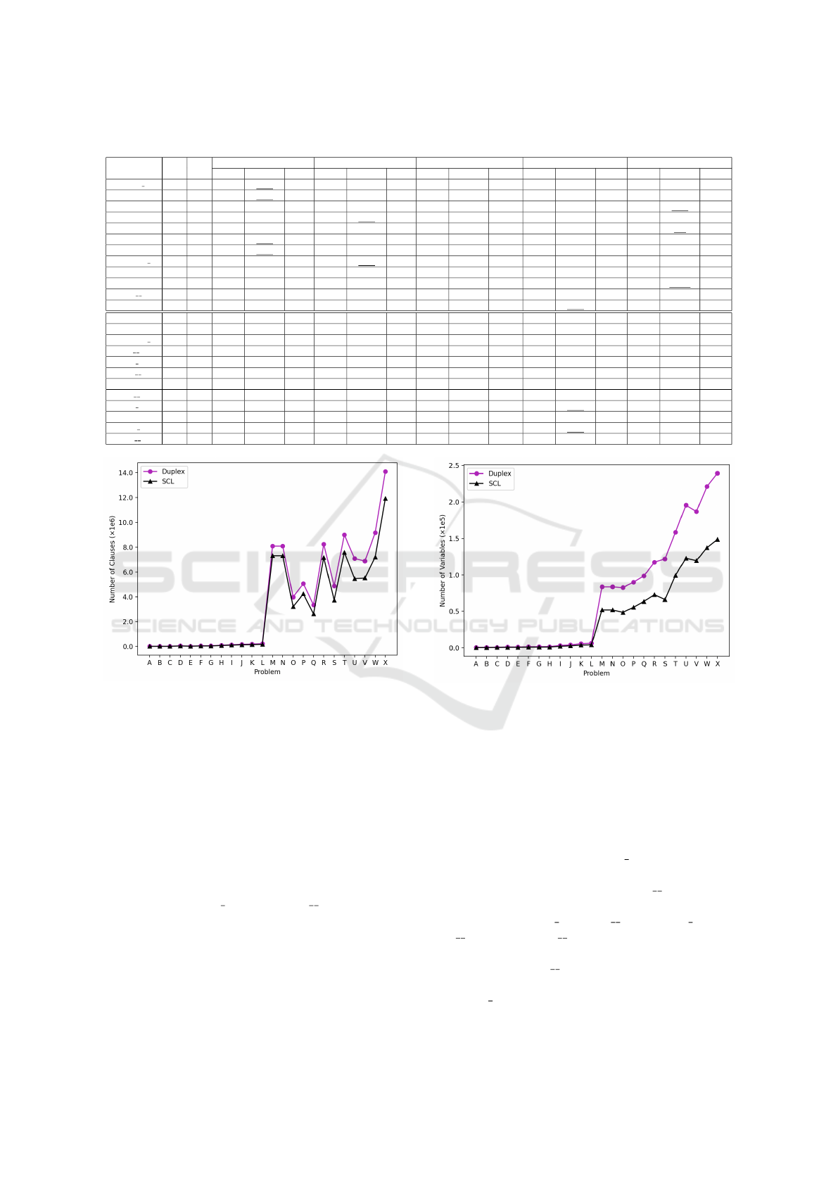
Table 3: ABP solving results with TO = 1800s and MO = 30GB.

Instance LB UB

Duplex SCL F

(k) CP-CPLEX CP-MZ-Chuffed

Obj-k Time(s) MB Obj-k Time(s) MB Obj-k Time(s) MB Obj-k Time(s) MB Obj-k Time(s) MB

A-pores 1 6 8 6 3.40 14.1 6 3.48 12.6 6 3.53 74.9 7 TO 579.3 6 4.75 42.3

B-ibm32 9 9 9 0.19 8.8 9 0.3 7.8 9 4.57 106.8 9 0.39 41.3 9 1.06 29.3

C-bcspwr01 16 17 17 1.11 11.2 17 4.19 18.6 17 3.59 97.5 17 0.67 41.0 17 0.43 28.6

D-bcsstk01 8 9 9 0.54 14.9 9 0.19 12.6 9 14.9 147.0 9 2.28 46.8 9 1.12 41.0

E-bcspwr02 21 22 21 2.15 14.9 21 1.52 11 21 17.8 170.2 21 15.83 51.5 21 0.8 31.5

F-curtis54 12 13 13 0.27 14.1 13 0.28 12.3 13 13.3 145.8 13 2.5 47.2 13 1.35 38.8

G-will57 12 14 13 0.29 14.4 13 0.47 13.9 13 18.5 175.6 13 14.18 51.5 13 1.09 39.9

H-impcol b 8 8 8 0.26 21.0 8 0.23 16.8 8 3.12 167.4 8 0.32 44.7 8 0.86 55.5

I-ash85 19 27 24 TO 272 24 TO 381 22 TO 460.3 23 TO 288.2 23 TO 374.8

J-nos4 32 40 35 472 177 35 980 503 - TO 927.0 35 TO 272.7 35 384.4 343.9

K-dwt 234 46 58 51 TO 685 51 TO 530 50 TO 895.3 52 TO 243.8 47 TO 244.6

L-bcspwr03 39 39 39 0.58 53 39 0.69 40.9 39 11.15 559.0 39 0.25 48.2 39 2.34 66.6

M-bcsstk06 28 72 35 TO 1726 35 TO 1398 - TO 12207 30 TO 738.4 - TO 3016

N-bcsstk07 28 72 35 TO 1726 35 TO 1397 - TO 12244 30 TO 737.9 - TO 3016

O-impcol d 91 173 101 TO 1745 102 TO 1802 - - MO 121 TO 491.3 - TO 1410

P-can 445 78 120 - TO 2464 79 TO 2156 - - MO 79 TO 869.2 - TO 1843

Q-494 bus 219 246 - TO 1443 220 TO 1301 - TO 23775 220 TO 701.6 - TO 763.8

R-dwt 503 46 71 64 TO 1634 64 TO 1474 - TO 10633 56 TO 717.6 - TO 1950

S-sherman4 256 272 - TO 1326 - TO 1073 - - MO - TO 689.9 - TO 888.8

T-dwt 592 103 150 - TO 5357 104 TO 2619 - - MO 104 TO 1366 - TO 1905

U-662 bus 219 220 220 471 2498 220 144 1377 - - MO 220 3.15 250.4 - TO 1061

V-nos6 326 337 - TO 1836 - TO 1532 - - MO - TO 967.9 - TO 1168

W-685 bus 136 136 136 10.7 1431 136 7.57 1164 - - MO 136 1.95 332.6 - TO 1325

X-can 715 112 142 - TO 3060 113 TO 4599 - - MO 113 TO 1380 - TO 2442

Figure 7: Comparison of the number of clauses between

Duplex and SCL.

ings are not included in Table 3. For each problem, the

table includes the best solution identiﬁed by each ap-

proach, the solving time (in seconds), and the memory

consumption (in MB). The best anti-bandwidth value

is highlighted in bold, while the best solving time is

underlined.

Figures 7 and 8 illustrate the comparison of the

number of clauses and auxiliary variables utilized in

the ABP encoding across 24 problems, evaluated us-

ing both the SCL and Duplex encodings. Each prob-

lem is represented by the ﬁrst letter of its name (A for

the problem A-pores 1, X for X-can 715). We ana-

lyze the encodings achieved at the maximum width

that both methods can solve within speciﬁed time

and memory limits. The results indicate that as the

problem size increases, SCL requires fewer clauses

and auxiliary variables than Duplex. This evidence

demonstrates why SCL can outperform Duplex in

Figure 8: Comparison of the number of variables between

Duplex and SCL.

solving certain ABPs, particularly in challenging sce-

narios characterized by a high number of edges and

vertices in the 12 larger graphs, as well as in terms of

memory usage.

In the 12 relatively small to medium-sized graphs,

both SCL and Duplex demonstrate competitive per-

formance, generally surpassing other methods. Com-

pared to the best CP approach, SCL outperforms CP-

CPLEX in the problems A-pores 1, I-ash85, and J-

nos4. However, CP-CPLEX performs better than

SCL and Duplex in the problem K-dwt 234. Among

the 12 larger graphs, SCL outperforms Duplex in 5

problems: O-impcol d, P-can 445, Q-494 bus, T-

dwt 592, and X-can 715. Additionally, SCL ex-

ceeds CP-CPLEX in 3 problems: M-bcsstk06, N-

bcsstk07, and R-dwt 503. Nonetheless, CP-CPLEX

achieves signiﬁcantly outperforms SCL in the problem

O-impcol d. When solving UNSAT instances, CP-

Sequential Counter Encoding for Staircase At-Most-One Constraints

173

CPLEX is weaker than both SCL and Duplex in cases

such as A-pores 1 (UNSAT with a width of 17), E-

bcspwr02 (UNSAT with a width of 22), and G-will57

(UNSAT with a width of 14).

5.4 Summary

Our proposed encoding, SCL, offers a valuable solu-

tion for addressing various SCAMO and ABP prob-

lems. In terms of SCAMO encoding, SCL outper-

forms all other SAT encodings regarding the number

of clauses, auxiliary variables, and solving time. For

ABP problems, SCL either matches or exceeds opti-

mal values in many instances, while demonstrating

competitive time efﬁciency and low memory usage.

Its ability to ﬁnd valid solutions in complex instances

where other encodings timeout underscores its robust-

ness and scalability. Experimental results show that

SCL surpasses Duplex, which is recognized as an efﬁ-

cient encoding for SCAMO and ABP (Fazekas et al.,

2020). Additionally, SCL outperforms CP-CPLEX, a

well-known commercial tool developed by IBM; SCL

exceeds CP-CPLEX in 6 out of 24 problems, while

CP-CPLEX only surpasses SCL in 2 out of 24 prob-

lems. Overall, SCL effectively balances performance

with resource management, making it a strong option

for tackling SCAMO and ABP challenges.

6 CONCLUSIONS

The paper presents our proposed SAT encoding for

SCAMO constraints, named SCL encoding. It uti-

lizes Sequential Counter Encoding for at-most-one

constraints with a staircase shape. SCL requires fewer

auxiliary variables and generates fewer clauses, mak-

ing it effective for encoding SCAMO constraints. It

yields better results for the anti-bandwidth problem

compared to other SAT encoding techniques as well

as Constraint Programming (CP) and Mixed Integer

Programming (MIP) approaches. Our proposed en-

coding, SCL, provides an efﬁcient encoding for other

combinatorial problems that involve SCAMO con-

straints.

ACKNOWLEDGEMENTS

We thank the authors of Duplex encoding (Fazekas

et al., 2020) for publishing the source code of Du-

plex, which allows us to implement the Antiband-

width problem more conveniently. This work has

been supported by VNU University of Engineering

and Technology under project number CN24.10.

REFERENCES

ıo, I., Nieuwenhuis, R., Oliveras, A., Rodr

ıguez-

Carbonell, E., and Mayer-Eichberger, V. (2012). A

new look at bdds for pseudo-boolean constraints.

Journal of Artiﬁcial Intelligence Research, 45:443–

480.

Akers (1978). Binary decision diagrams. IEEE Transac-

tions on computers, 100(6):509–516.

Artigues, C., Hebrard, E., Mayer-Eichberger, V., Siala, M.,

and Walsh, T. (2014). Sat and hybrid models of the

car sequencing problem. In Integration of AI and OR

Techniques in Constraint Programming: 11th Inter-

national Conference, CPAIOR 2014, Cork, Ireland,

May 19-23, 2014. Proceedings 11, pages 268–283.

Springer.

Bessiere, C., Hebrard, E., Hnich, B., Kiziltan, Z., Quim-

per, C.-G., and Walsh, T. (2007). Reformulating

global constraints: The slide and regular constraints.

In Abstraction, Reformulation, and Approximation:

7th International Symposium, SARA 2007, Whistler,

Canada, July 18-21, 2007. Proceedings 7, pages 80–

92. Springer.

Biere, A. (2019). Cadical at the sat race 2019. In Heule, M.,

arvisalo, M., and Suda, M., editors, Proceedings of

SAT Race 2019: Solver and Benchmark Descriptions,

volume B-2019-1 of Department of Computer Science

Series of Publications B, University of Helsinki 2019,

pages 8–9.

Bryant, R. E. (1986). Graph-based algorithms for boolean

function manipulation. Computers, IEEE Transac-

tions on, 100(8):677–691.

Cappanera, P. (1999). A survey on obnoxious facility loca-

tion problems.

Ceschia, S., Dang, N. T. T., De Causmaecker, P., Haspes-

lagh, S., and Schaerf, A. (2015). Second in-

ternational nurse rostering competition (inrc-ii)—

problem description and rules—. arXiv preprint

arXiv:1501.04177.

Chen, J. (2010). A new sat encoding of the at-most-one con-

straint. Proc. constraint modelling and reformulation,

page 8.

Duarte, A., Mart

ı, R., Resende, M. G., and Silva, R. M.

(2011). Grasp with path relinking heuristics for the

antibandwidth problem. Networks, 58(3):171–189.

Fazekas, K., Sinnl, M., Biere, A., and Parragh, S. (2020).

Duplex encoding of staircase at-most-one constraints

for the antibandwidth problem. In International

Conference on Integration of Constraint Program-

ming, Artiﬁcial Intelligence, and Operations Re-

search, pages 186–204. Springer.

Gent, I. P., Petrie, K. E., and Puget, J.-F. (2006). Symmetry

in constraint programming. Foundations of Artiﬁcial

Intelligence, 2:329–376.

Haberlandt, A., Green, H., and Heule, M. J. (2023). Ef-

fective auxiliary variables via structured reencoding.

arXiv preprint arXiv:2307.01904.

Hale, W. K. (1980). Frequency assignment: Theory and

applications. Proceedings of the IEEE, 68(12):1497–

1514.

ICAART 2025 - 17th International Conference on Agents and Artiﬁcial Intelligence

174

Hu, Y., Gansner, E. R., and Kobourov, S. (2010). Visual-

izing graphs and clusters as maps. IEEE Computer

Graphics and Applications, 30(6):54–66.

Kletzander, L. and Musliu, N. (2020). Solving the general

employee scheduling problem. Computers & Opera-

tions Research, 113:104794.

Leung, J. Y., Vornberger, O., and Witthoff, J. D. (1984). On

some variants of the bandwidth minimization prob-

lem. SIAM Journal on Computing, 13(3):650–667.

Nethercote, N., Stuckey, P. J., Becket, R., Brand, S., Duck,

G. J., and Tack, G. (2007). Minizinc: Towards a stan-

dard cp modelling language. In International Con-

ference on Principles and Practice of Constraint Pro-

gramming, pages 529–543. Springer.

Nieuwenhuis, R., Oliveras, A., Rodr

ıguez-Carbonell, E.,

and Rollon, E. (2021). Employee scheduling with sat-

based pseudo-boolean constraint solving. IEEE ac-

cess, 9:142095–142104.

Rodriguez-Tello, E., Romero-Monsivais, H., Ram

ırez-

Torres, J., and Lardeux, F. (2015). Harwell-boeing

graphs for the cb problem.

Siala, M. (2015). Search, propagation, and learning in se-

quencing and scheduling problems. PhD thesis, INSA

de Toulouse.

Sinnl, M. (2021). A note on computational approaches for

the antibandwidth problem. Central European Jour-

nal of Operations Research, 29(3):1057–1077.

Sinz, C. (2005). Towards an optimal cnf encoding of

boolean cardinality constraints. In International con-

ference on principles and practice of constraint pro-

gramming, pages 827–831. Springer.

Vasconcellos-Gaete, C., Barichard, V., and Lardeux, F.

(2020). Abacus: A new hybrid encoding for sat prob-

lems. In 2020 IEEE 32nd International Conference on

Tools with Artiﬁcial Intelligence (ICTAI), pages 145–

152. IEEE.

APPENDIX

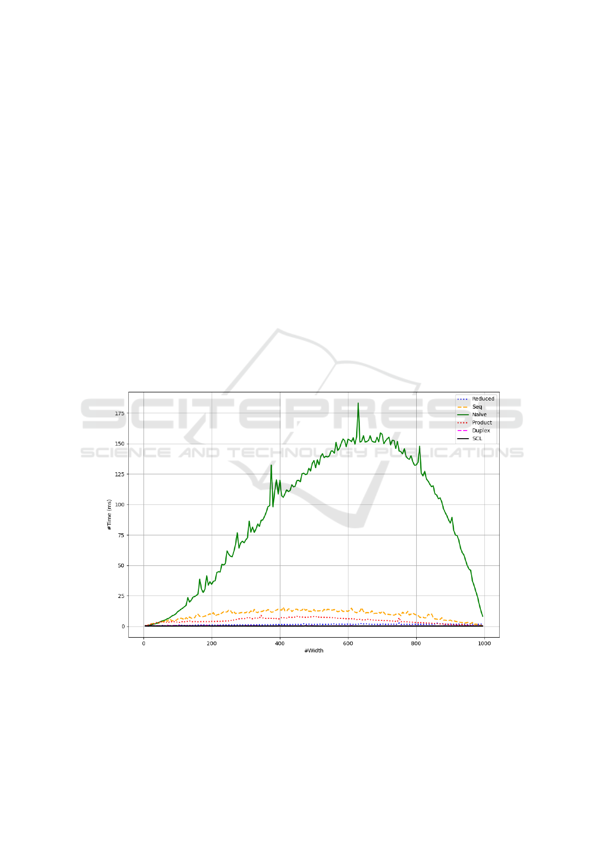
Figure 9 shows the time taken (in milliseconds) by

the Reduced, Seq, Naive, Product, Duplex, and SCL

encodings for the SCAMO problem, where n = 1000

and w ranges from 1 to 1000 in increments of 5.

Figure 9: Comparison of solving time of different encodings in SCAMO with parameters set to n = 1000 and w ∈(1, 1000).

Sequential Counter Encoding for Staircase At-Most-One Constraints

175