3D View Reconstruction from Endoscopic Videos for Gastrointestinal

Tract Surgery Planning

Xiaohong W. Gao

, Annisa Rahmanti

and Barbara Braden

Department of Computer Science, Middlesex University, London, U.K.

Medical Department B, University of Münster, Germany

Keywords: Deep Learning, 3D Reconstruction, Nerfs, Gastrointestinal Tract, SfM, 2D Endoscopic Video, Endoscopic

Artefacts.

Abstract: This paper investigates the application of neural radiance field (NeRF) to reconstruct a 3D model from 2D

endoscopic videos for surgical planning and removal of gastrointestinal lesions. It comprises three stages. The

first one is video preprocess to remove frames with artefact of colour misalignment based on a deep learning

network. Then the remaining frames are converted into NeRF compatible format. This stage includes

extraction of camera information regarding intrinsic, extrinsic and ray pathway parameters as well as

conversion to NeRF format based on COLMAP library, a pipeline built upon structure-from-motion (SfM)

with multi-view stereo (MVS). Finally the training takes place for establishment of NeRF model implemented

upon Nerfstudio library. Initial results illustrate that this end-to-end, i.e. from 2D video input to 3D model

output deep learning architecture presents great potentials for reconstruction of gastrointestinal tract. Base on

the two sets of data containing 2600 images, the similarity measures of SSIM, PSNR and LPIPS between

original (ground truth) and rendered images are 19.46 ± 2.56, 0.70 ± 0.054, and 0.49 ± 0.05 respectively.

Future work includes enlarging dataset and removal of ghostly artefact from rendered images.

1 INTRODUCTION

Gastrointestinal tract (GI) cancers (oesophagus,

stomach, bowel), were responsible for 26.3% of

cancer cases and 35.4% of deaths worldwide in 2018

(Lu 2021). As the 2

largest death caused by cancer

in the world (after lung cancer), GI cancers have very

low 5-year survival rate (<20%). At present, the only

curative and most effective treatment for early GI

cancer or lesion is the removal of concerned lesion

endoscopically, especially, for a lesion confined to the

mucosal layer, the surface columnar epithelium and

the first of four layers on the GI wall. In this

procedure, a substance is injected first under the target

to act as a cushion. Then a surgical plan by marking

cutting lines is conducted. Finally, the dissection takes

place at submucosal layer under the concerned lesion

following the planning boundary. The key to success

of this surgery is that the endoscopists have a clear

view of the lesion, the planned lines and surroundings

https://orcid.org/0000-0002-8103-6624

https://orcid.org/0000-0001-9478-6267

https://orcid.org/0000-0002-8534-6873

from varying view angles throughout in order to

perform precise dissection.

The challenges here are that all the views are

confined into a narrow (~2cm in diameter) cylindrical

food path or tube where the endoscopic camera travels

in one direction, resulting in some concerned tissues,

anatomy and planned boundary being invisible. In

addition, in this complex surgical scene, the

endoscopist/surgeon/clinician has to compete with

various motions coming from respiration, heartbeat,

camera as well as muscles. Because of this, at present,

all these operations can only be conducted by expert

endoscopists, which put significant amount of pressure

in health care systems. Figure 1 demonstrates the

process of resection of a polyp in the stomach

endoscopically. While the lesion in Figure 1 is benign,

if left untreated, it could progress into cancer. Hence

resection is in need. Once the target is confirmed

(Figure 1 (a)), an injection of a dedicated substance is

carried out to highlight and alleviate the lesion whereby

Gao, X. W., Rahmanti, A. and Braden, B.

3D View Reconstruction from Endoscopic Videos for Gastrointestinal Tract Surgery Planning.

DOI: 10.5220/0013125000003911

Paper published under CC license (CC BY-NC-ND 4.0)

In Proceedings of the 18th International Joint Conference on Biomedical Engineering Systems and Technologies (BIOSTEC 2025) - Volume 1, pages 221-228

ISBN: 978-989-758-731-3; ISSN: 2184-4305

221

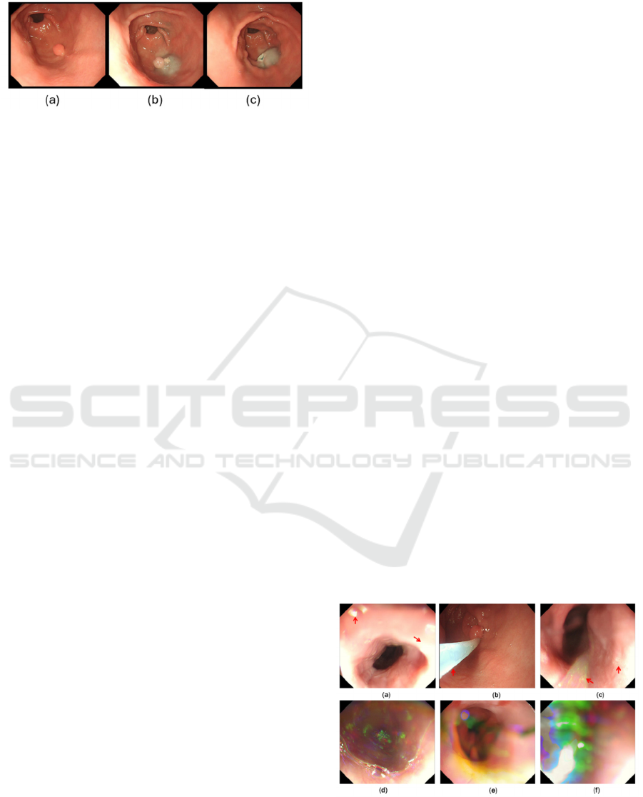
a surgical planning can be made (Figure 1(b)). Then the

lesion can be removed safely (Figure 1(c)).

Figure 1: Demonstration of lesion resection endoscopically.

(a) a lesion is detected; (b) cushion is injected; (c) successful

removal of the concerned lesion.

Hence reconstruction of 3D view of concerned

lesions plays an important role in endoscopic surgical

planning and lesion removal. 3D reconstruction for GI

from endoscopic videos has been studied by a number

of researchers. For example, Ali et al (Ali 2021a) has

established a physical model of oesophagus that is

applied to develop an AI system to quantify Barrett’s

oesophagus. The researchers as detailed in (Prinzen,

2015) has been established the shape of oesophagus to

allow visualization of additional contextual and

geometrical information of oesophagus, from

panorama image to 3D points cloud then to regular

triangulation mesh. Recently, 3D shape reconstruction

of whole stomach based on structure-from-motion

(SfM) (Widya 2019) is investigated by spreading

indigo carmine (IC) dye on the stomach surface to

present colour texture of the stomach. This is because

endoscopic videos present weak texture of GI surface.

On the other hand, the approach of SfM appears to

present robust results when it comes 3D

reconstruction from 2D videos. Further study for deep

multi-view stereo for dense 3D reconstruction (Bae

2020) is also conducted based on SfM and is consisted

of 3 steps, which are sparse reconstruction via SfM,

monocular depth estimation and embedding vector

generation via patch embedding network.

The steps to construct a 3D model from 2D image

usually include image collection, feature or/and

keypoint detection and extraction, keypoint tracking

and matching, structure from motion to determine

camera intrinsic, extrinsic and orientation parameters,

and key point-cloud reconstruction, such as mesh

reconstruction, mesh refinement and mesh texturing.

With the current advances of state-of-the-art

(SOTA) deep learning (DL) techniques, many

innovative approaches have been developed towards

reconstructing 3D deformable objects.

In this study, 3D scene reconstruction based on 2D

endoscopic videos is conducted based on SOTA

neural radiance field (NeRF) so that a lesion can be

viewed from all viewing angles, allowing correct

recognition of concerned lesions, tissue types and

related anatomy, leading to an assistant system in an

operative room allowing multiple views while

performing lesion removal.

NeRF (Mildenhall 2020) addresses the long-

standing problem in computer vision field, which is to

reconstruct a 3D representation of a scene from sparse

2D images. NeRF method synthesizes a new view by

directly optimising parameters of a continuous 5D

scene representation to minimize the error of

rendering a set of captured images. NeRF represents

a scene using a fulling connected deep network with

an input of a single continuous 5D coordinate (i.e. 3D

spatial + 2D view direction angles). The output of this

network is the volume density and view-dependent

emitted radiance at that spatial location.

2 METHODOLOGY

2.1 Image Pre-Process to Remove

Artefact of Colour Misalignment

Due to the confinement of narrow space of GI, it is

quite common that as many as a quarter video frames

contain several types of artefacts, such as water

bubbles, instrument, and saturation. While these

artefacts are present most of the time, the concerned

image features are still visible. However, the artefact

of colour misalignment, where coloured frames of red,

green and blue are acquired at different locations

because of the combination of movements when an

endo camera travels, should be removed not only

because most of interested contents are not present but

also the presence of these artificial colours will affect

the detection of camera light of rays, hence affecting

the accuracy of training. Figure 2 illustrates a number

of artefacts present in a video clip, where the top row

Figure 2: Examples of frames with artefacts (arrow). (a)

saturation; (b) instrument; (c) bubbles; (d)(e)(f) colour

misalignment (all over images).

BIOIMAGING 2025 - 12th International Conference on Bioimaging

222

of artefacts (red arrows) still contains visible GI

features but bottom row of colour misalignment

(whole images) mis-represents GI contents.

To detect artefacts, many deep learning-based

systems are developed offering promising

performance (Ali 2020, Ali 2021b,

Bissoonauth-Daiboo

2023). In this study, the processing time also plays an

important role for the future development of real-time

3D systems. Hence the real-time system, real-time

instance segmentation system, YOLACT (Bolya

2019, Gao 2023) is enhanced and applied for artefact

classification. Figure 2 presents the architecture of the

network to classify frames with normal or artefact

features (instrument, bubbles, saturation or colour

misalignment (CMA)). In this pre-processing stage,

only frames with CMA will be discarded. This is

because the subsequent 3D modelling and

reconstruction of lesioned GI depends on the

information of colour and intensity attributes, i.e.

structure from motion and neutral radiance fields.

Figure 3: The architecture of YOLACT network for

detection and segmentation of artefact. The artefacts to

distinguish are instrument, bubbles, saturation, and colour

misalignment (CMA). The mask or ground truth of frames

with CMA is the whole frame.

For this end-to-end detection system of YOLACT

(Bolya 2019) (Figure 3), the basic underline model

employs ResNet101 to extract initial feature maps.

The object segmentation is accomplished through two

parallel subnets (ProtoNet and Prediction Head),

which generate a set of prototype masks and predict

per-object mask coefficients respectively.

More specifically, ProtoNet employs a fully

connected network (FCN) accommodating the largest

pyramid feature layer (𝑃3), to produce a set of image-

sized prototype masks. These 𝑘 mask prototypes (𝑘

32 in this study) are then applied to deliver predictions

for the entire image in relation to classification,

segmentation and detection (Gao 2023).

On the other hand, Prediction Head contains three

branches, which are c class confidence (c=5 for

‘Instrument’, ‘Bubbles’, ‘Saturation’, ‘artefact-text’,

‘CMA’), 4 bounding box regressors (=[x

top-left-corner

top-left-corner,

width, height])), and a vector of mask

coefficients, one for each prototype to be processed in

parallel. Subsequently, the branch of

‘Crop+thresholding’ in Figure 2 delivers a vector size

of 4  𝑐  𝑘 for each anchor or region of interest

(RoI), As a result, for each instance, one or more

masks will stem from that instance by linearly

combining (plus or minus) the work from both

prototype and mask coefficient strands, leading to the

production of final masks ( 𝑀 ) by a sigmoid

nonlinearity as formulated in Eq. (1).

𝑀𝜎𝑃𝐶



 (1)

where 𝑃 is an ℎ𝑤𝑘 matrix of prototype masks

and 𝐶 is a 𝑛  𝑘 matrix of mask coefficients for 𝑛

instances that have passed score thresholding and

initial 𝑁𝑀𝑆 , the maxima suppression technique

(Bolya 2019). NMS determines whether an instance

should be kept or discard. For example, duplicated

detections are suppressed not only for the same class

but also for cross-class boundary boxes depending on

the probability of boxes, i.e. the box with higher

probability suppresses the one with lower

probability. In Eq. (1), 𝐶



indicates the transpose of

𝐶 Matrix.

The calculation of the loss function is the same as

for YOLACT (Bolya 2019). Three loss functions are

utilised to train this end-to-end detection model as

formulated in Eq. (2), which are classification loss

(ℒ



, box regression loss ( ℒ



 and mask loss

ℒ



 where the weights of 1, 1.5, and 1.5 are

applied for them respectively to give more weight to

classification.

ℒℒ



1.5 ℒ



1.5 ℒ



(2)

In particular,

ℒ



𝐵𝐶𝐸𝑀,𝑀



 (3)

where the binary cross entropy 𝐵𝐶𝐸 is formulated

using Eq. (4).

𝐵𝐶𝐸𝑝, 𝑦  





∑

𝑦



log



𝑝





1





𝑦



log 1  𝑝





(4)

where 𝑦 represents the label and 𝑝 is the predicted

probability of the point being a label for all 𝑁 points.

𝑀 and 𝑀



are calculated in Eq. (1).

After removing the frames with CMA artefact, the

remaining are applied to train the 3D model takes

place based on NeRF.

3D View Reconstruction from Endoscopic Videos for Gastrointestinal Tract Surgery Planning

223

2.2 3D View Reconstruction for

Concerned Lesioned GI Based on

NeRF

For 3D scene modelling, neural radiance fields

(NeRFs) (Mildenhall 2020) takes 5-degree

coordinates as an input. The 5D refer to each 3D point

at (𝑥, 𝑦,𝑧) when viewing with a camera ray of light

emitting direction at (𝜃, 𝜙). Hence, NeRF enables

learning novel view synthesis, scene geometry and

reflectance properties by optimising a deep fully-

connected neural network as a multilayer perceptron

(MLP). As such, NeRF represents this 5D function by

regressing from a single 5D coordinate (𝑥,𝑦,𝑧,𝜃,𝜙

to a single volume density and view-dependent RGB

colour. As a result, to render NeRF from a specific

viewpoint, camera rays are marched through the

scene, and a neural network produces colours and

densities for 3D points, which are then accumulated

into a 2D image.

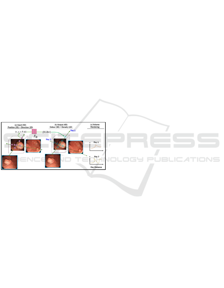
Figure 4 schematically illustrates the process of

representing scenes as neural radiance fields for view

synthesis.

Figure 4: The process flow of NeRF. (a) 5D input; (b) 4D

output; (c) volume rendering at a new viewing direction.

Firstly, a scene (Figure 4(a)) is represented using a

5D vector-valued function with an input of a 3D

location 𝒙  𝑥,𝑦,𝑧 and 2D viewing direction 𝒅 

𝜃,𝜙. The output of this function is an emitted colour

𝒄 𝑟,𝑔,𝑏 and volume density



(Figure 4(b)) at

each ray. This 5D function is approximated applying

a multilayer perceptron (MLP) network 𝐹





𝒙, 𝒅



→

𝒄, 𝝈 to optimise its weights



in order to map each

input 5D coordinate to its corresponding volume

density and directional emitted colour. Finally, based

on the classical volume rendering approach (Kajiya

1984), the colour of any light ray passing through the

scene is rendered (Figure 4(c)) whereas the volume

density 𝝈𝒙 is interpreted as the differential

probability of a ray terminating at location 𝒙. Hence

the expected colour 𝐶𝒓 of camera ray light 𝒓



𝑡





𝒐𝑡𝒅 , starting at the original location 𝒐, with near

and far bounds 𝑡



and 𝑡



, is expressed in Eq. (5)

(Mildenhall 2020).

𝐶



𝑟







𝑇



𝑡



𝜎𝒓



𝑡



𝑐



𝒓



𝑡



,𝒅



𝑑𝑡









(5)

where

𝑇



𝑡



exp 



𝜎





𝒓



𝑠



𝑑𝑠 (6)

As pointed out by Mildenhall et al [6], operating a

network 𝐹



directly on 𝑥𝑦𝑧𝜃𝜙 can result in poorly

rendering performance when colour and geometry

have high-frequency variations. Hence, 𝐹



formulated as a composite of two functions, i.e., 𝐹





𝐹





∘𝛾

, where 𝐹





is learned applying a regular MLP

network, from which the estimated colour 𝐶







𝒓



can

be expressed in Eq. (7) as a weighted sum of all

sampled colours 𝑐



along the ray.

𝐶







𝒓





∑

𝑤



𝑐









(7)

where

𝑤



𝑇



1  exp



𝜎



𝛿





 (8)

𝑇



exp

∑

𝜎



𝛿







 (9)

and

𝛿



𝑡



𝑡



(10)

𝛿



in Eq (10) refers to the distance between adjacent

samples.

On the other hand, 𝛾

is not learnt but a mapping from

ℝ space into a higher dimensional space ℝ



computed in Eq. (11).

𝛾



𝑝



 sin





𝜋𝑝



, cos





𝜋𝑝



, … , sin





𝜋𝑝



,cos 2



𝜋𝑝

(11)

Where 𝑝 𝑥,𝑦,𝑧,𝜃,𝜙 respectively. 𝐿 10 when

𝑝 𝑥,𝑦,𝑧,𝜃,𝜙 and 𝐿 4 when 𝑝 𝜃,𝜙 .

Hence the loss between ground true colour 𝐶𝒓)

and predicted pixel colours for both coarse 𝐶







𝒓



and

fine 𝐶







𝒓



renderings is calculated in Eq. (12).

ℒ 

∑

𝐶







𝒓



𝐶𝒓





∈ℛ

𝐶







𝒓



𝐶𝒓





(12)

where ℛ is the set of rays in each batch.

2.3 Implementation

To model 3D view of endoscopic view based on

NeRFs, Nerfstudio (Tancik 2023) is implemented.

Nerfstudio tools are a repository collecting an family of

simple python-based extensive application programing

interface (API) functions to allow visualisation of

modelling of scenes based on neural radiance fields

BIOIMAGING 2025 - 12th International Conference on Bioimaging

224

(NeRFs). By providing a simplified end-to-end process

of creating, training and testing NeRFs, these APIs

allow viewing and interacting these processes through

an internet browser.

In this study, the input data are a clip of endoscopic

video containing RGB frames. After removal of

artefact of CMA as explained in Section A, these

frames/images are analysed to extract needed

information, including ground truth information such as

camera intrinsic and extrinsic data. To obtain the

endoscopic camera information, COLMAP system is

employed. COLMAP (

Schonberger 2016)

is the

structure-from-motion (SfM) package that can be

employed to estimate the ground truth information

regarding to camera poses, camera intrinsic parameters,

and scene boundaries. In addition, this pre-processing

stage converts those input images into a format that is

compatible with NerfStudio

, i.e. a JSON format.

Then training takes place based on the pre-

processed images to create a configuration file and a

model.

2.4 Similarity Measurements

Three common measures are employed to calculate

the similarity between original (ground truth) and

rendered images, which are structural similarity

(SSIM) (Wang 2004) (Eq. (13)), peak signal-to-noise

ratio (PSNR) (Eq. (14)), and more recently Learned

Perceptual Image Patch Similarity (LPIPS) (Eq.(15)).

𝑆𝑆𝐼𝑀



𝑥,𝑦



















,









































(13)

In Eq. (13) of SSIM, 𝜇



,𝜇



are the averages of 𝑥,

𝑦 , with 𝜎





,𝜎





being the variances of 𝑥

, 𝑦

respectively and 𝜎

,

the covariance of 𝑥

and 𝑦. The

variables of 𝑐



and 𝑐



are applied to stabilize the

division when a small denominator occurs and are set

to be 0.01𝐿



and 0.03𝐿



respectively, whereby L

stands for the dynamic intensity range of an image,

e.g. L=255 for an 8-bit image. 𝑥

,𝑦 refer to original

and rendered images respectively.

For PSNR, Eq. (14) is calculated.

𝑃𝑆𝑁𝑅  20log



𝑀𝐴𝑋



10log



𝑀𝑆𝐸 (14)

where 𝑀𝐴𝑋



refers to the maximum possible value of

the image (e.g. 255 for 8-bit) and 𝑀𝑆𝐸 the mean

squared error between two concerned images.

In addition, LPIPS (Zhang 2018) metric refers to

Learned Perceptual Image Patch Similarity and is

formulated in Eq. (15). LPIPS is calculated by

comparing the activations of two image patches using

pre-defined neural network features. Specifically, it

https://docs.nerf.studio.

computes the distance between the feature

representations of the patches. The lower the LPIPS

score is, the more perceptually similar the patches are.

The distance between reference and rendered

patches 𝑥, 𝑥



with network ℱ is calculated in Eq. (15)

where 𝐻,𝑊,𝐶 refer to image patch high, width, and

channel.

𝑑



𝑥,𝑥







∑











∑

𝑤



⊙𝑦





𝑦













,

(15)

The feature stacks are extracted from layer 𝐿

where unit-normalization ( 𝑦

, 𝑦





corresponding to

𝑥,𝑥



respectively) in the channel dimension takes

place, and for layer 𝑙 , 𝑦



, 𝑦







∈ℝ













. The

weight 𝑤



is performing element-wise multiplication

(⨀, which is equivalent to computing cosine distance

(Zhang 2018).

3 RESULTS

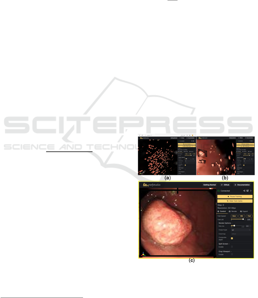
Figure 5 demonstrates the training processing

implemented via Nerfstudio. The training processing

is visualised live on a browser, which allows users to

select any camera ray direction as exemplified at

Figure 5 (a)(b) to view detailed training (5(a)) as well

as each individual training image (5(b)) with a specific

camera location (Figure 5(c)).

Figure 5: The illustration of training process. (a)(b) training

takes place at varying camera rays. (c) An individual

training sample selected from (b) with a specific camera ray

direction.

3D View Reconstruction from Endoscopic Videos for Gastrointestinal Tract Surgery Planning

225

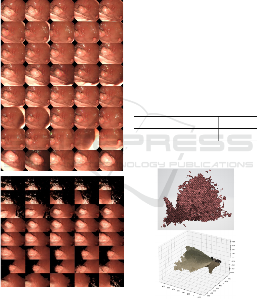
Figure 6 demonstrates the montage of training data

set (a) and the new view angle (b) rendered using the

trained model. The needed view path can be selected,

defined or requested through the visualisation tool

presented in Figure 5.

(a)

(b)

Figure 6: Demonstration of training data (a) and rendered

data (b) at a specific view direction for a polyps in the

stomach.

While the rendered data (Figure 6(b)) have some

background information missing due to the lack the

sufficient data, the concerned lesion can be rendered

and viewed at any needed viewing angle, which is

important in a clinical setting as an endoscopic camera

can only travel in one direction within the narrow food

path whereas clinicians need to know all the

surrounding information for a surgical planning.

The accuracy of rendered images using the

aforementioned three metric measures is provided in

Table 1, which is based on two sets of data. The initial

video frames with 10 minutes each contains over

30,000 frames each. After pre-process for detection of

colour misalignment artefact, 6000 frames are kept.

When extracting camera ray information using

COLMAN approach, only 2600 images are found

related due to poor image quality, e.g. blurry with

floating objects or noise/artefact.

Table 1: The measurement of similarity between ground

truth (original) and rendered images. for psnr and ssim,

higher value implies more similar whereas lower lpips

referring more similar between the two.

Data

set

Image

number

PSNR SSIM

LPIPS

2 2600 19.46 ±

2.56

0.70 ±

0.054

0.49 ±

0.05

Figure 7 presents a mesh and point cloud for the

concerned lesion shown in Figure 5, which can be

views at any viewing angle or camera light ray.

Figure 7: Demonstration of mesh (top) and point cloud

(bottom) of the concerned lesion shown in Figure 5.

BIOIMAGING 2025 - 12th International Conference on Bioimaging

226

4 CONCLUSION

This study investigates the feasibility of

reconstruction of 3D scene of GI from 2D endoscopic

videos as an end-to-end process, i.e. from an input 2D

video to an output 3D model, without the prior

knowledge of camera information of location,

intrinsic and extrinsic data. SOTA NeRF approach is

applied. Because of the challenges facing acquisition

of endoscopic video with less texture information on

the GI surface, the camera positional information

extracted from videos requires images with varying

view angles, which in our case, is limited. Hence the

ground truth images after pre-processing only contain

10% of the original input. However, even with only

1000 images for each lesion as one training dataset,

the 3D model is able to render high quality images

with various viewing angles. For the two training data

sets, the averaged measures of SSIM, PSNR and

LPIPS between original (ground truth) and rendered

images are 19.46 ± 2.56, 0.70 ± 0.054, and 0.49 ± 0.05

respectively. In comparison with the work of NeRF

where 31.01, 0.947 and 0.081 are obtained for natural

images [6], our results appear to be less performed.

However, in [6], around 100 views are acquired for

each filmed object with known camera information. In

our study, this information has to be extracted from

endoscopic videos themselves with much less viewing

angles due to the constraints of viewing space in the

food passage, leading to less image frames are

employed. In addition, because of the combination of

movements while performing endoscopic filming,

including heartbeat, respiration, and camera, many

images appear blurry to a certain extent. These blurry

images are usually ignored when applying COLMAP

library to track camera locations. This is because the

tracking of motion based on optical flow, i.e. the same

spot would appear similar intensity level in the

subsequent images, which is not the case for blurry

images.

In the future, more datasets will be evaluated. In

addition, post processing will be conducted including

to remove noises or ghostly artefact as recommended

more recently by Warburg et al (Warburg 2023).

Specifically, to make use as many video frames as

possible, especially for medical applications with

limited dataset, a new algorithm will be developed to

establish camera information based on the existing

available but less clear images through the application

of human vision models. While many frames are burry

with regard to motion tracking, human vision can still

perceive these motions easily and clearly. In this way,

the developed system will also become more

transparent.

ACKNOWLEDGEMENTS

This project is founded by the British Council as

Women in STEM Fellowship (2023-2024). Their

financial support is greatly acknowledged.

REFERENCES

Ali S, Zhou F, Braden B, et al (2020), “An objective

comparison of detection and segmentation algorithms

for artefacts in clinical endoscopy,” Nature Scientific

Reports, 10, Article number: 2748.

Ali S, Bailey A, Ash S, et al. (2021a), “A Pilot Study on

Automatic Three-Dimensional Quantification of

Barrett’s Esophagus for Risk Stratification and Therapy

Monitoring”, Gastroenterology, 161: 865-878.

Ali S, Dmitrieva M, Ghatwary N, et al (2021b), “Deep

learning for detection and segmentation of artefact and

disease instances in gastrointestinal endoscopy,”

Medical Image Analysis, 70:102002.

Bae G, Budvytis I, Yeung CK, Cipolla R (2020), “Deep

Multi-view Stereo for Dense 3D Reconstruction from

Monocular Endoscopic Video”, MICCAI 2020. Lecture

Notes in Computer Science, vol 12263. Springer.

Bissoonauth-Daiboo P, Khan MHM, Auzine MM, Baichoo

S, Gao XW, Heetun Z (2023), “Endoscopic Image

classification with Vision Transformers,” in ICAAI

2023, pp. 128-132.

Bolya D, Zhou C, Xiao F, Lee YJ (2019), YOLACT: real-

time Instance Segmentation, Proceedings of the ICCV

2019.

Gao XW, Taylor S, Pang W, Hui R , Lu X, Braden B (2023),

“Fusion of colour contrasted images for early detection

of oesophageal squamous cell dysplasia from

endoscopic videos in real time , Information Fusion,” 92:

64-79.

Kajiya JT, Herzen BPV (1984), “Ray tracing volume

densities,” Computer Graphics, SIGGRAPH.

Lu L, Mullins CS, Schafmayer C, Zeißig S, Linnebacher M

(2021), “A global assessment of recent trends in

gastrointestinal cancer and lifestyle-associated risk

factors,” Cancer Commun (Lond), 41(11): 1137-1151.

Mildenhall B, Srinivasan PP, Tancik M, et al. (2020), NeRF:

Representing Scenes as Neural Radiance Fields for

View Synthesis, in ECCV 2020.

Prinzen M, Trost J, Bergen T, Nowack S, Wittenberg T

(2015), “3D Shape Reconstruction of the Esophagus

from Gastroscopic Video,” In: H Handels, et al. (eds)

Image Processing for Medicine, pp. 173-178. Springer

Berlin, Heidelberg.

Schonberger JL, Frahm JM (2016), “Structure-from-motion

revisited,” In: CVPR’2016.

Tancik M, Weber E, Ng E, et al (2023), Nerfstudio: a

Modular Framework for Neural Radiance Field

Development, arXiv:2302.04264.

Wang Z, Bovik AC, Sheikh HR, Simoncelli EP (2004),

“Image quality assessment: From error visibility to

3D View Reconstruction from Endoscopic Videos for Gastrointestinal Tract Surgery Planning

227

structural similarity,” IEEE Transactions on Image

Processing, 13 (4) : 600-612.

Warburg F, Weber E, Tancik M, Hołyński A, Kanazawa A

(2023),” Nerfbusters: Removing Ghostly Artifacts from

Casually Captured NeRFs,” ICCV’2023.

Widya A, Monno Y, Imahori K, et al (2019), “3D

reconstructor of whole stomach from endoscope video

using structure-from-motion”, arXiv:1905,12988v1.

Zhang R, Isola P, Efros AA, Shechtman E, Wang O (2018),

“The unreasonable effectiveness of deep features as a

perceptual metric,” In: CVPR’2018.

BIOIMAGING 2025 - 12th International Conference on Bioimaging

228