Segment-Level Road Obstacle Detection

Using Visual Foundation Model Priors and Likelihood Ratios

Youssef Shoeb

1,3

, Nazir Nayal

, Azarm Nowzad

Fatma G

uney

and Hanno Gottschalk

Continental AG., Germany

Koc¸ University, Turkey

Technische Universit

at Berlin, Germany

Keywords:

Road Obstacle Detection, Likelihood Ratio, Applications of Foundational Models.

Abstract:

Detecting road obstacles is essential for autonomous vehicles to navigate dynamic and complex trafﬁc envi-

ronments safely. Current road obstacle detection methods typically assign a score to each pixel and apply a

threshold to generate ﬁnal predictions. However, selecting an appropriate threshold is challenging, and the

per-pixel classiﬁcation approach often leads to fragmented predictions with numerous false positives. In this

work, we propose a novel method that leverages segment-level features from visual foundation models and

likelihood ratios to predict road obstacles directly. By focusing on segments rather than individual pixels,

our approach enhances detection accuracy, reduces false positives, and offers increased robustness to scene

variability. We benchmark our approach against existing methods on the RoadObstacle and LostAndFound

datasets, achieving state-of-the-art performance without needing a predeﬁned threshold.

1 INTRODUCTION

Detecting road obstacles is critical for ensuring the

safe maneuvering of automated vehicles. Deep Neu-

ral Networks (DNNs) have demonstrated impressive

performance on various perception tasks in automated

driving, such as trafﬁc sign recognition, road segmen-

tation, and object detection. However, DNN-based

approaches tend to perform poorly on detecting ob-

jects not encountered in their training data (Nguyen

et al., 2015a). This presents a signiﬁcant safety con-

cern, as including all potential road obstacles in the

training data is impractical and can lead to potentially

hazardous situations on the road if a road obstacle is

missed.

For the task of semantic segmentation, learned

features are densely mapped to a pre-deﬁned set of

classes by a pixel-level classiﬁer, allowing for accu-

rately detecting and localizing every object in the im-

age. Since training a segmentation model for all pos-

sible road obstacles is infeasible, road obstacle de-

tection has been commonly addressed as an out-of-

distribution (OoD) detection task. Previous methods

for OoD detection in semantic segment networks have

primarily focused on per-pixel reasoning (Di Biase

et al., 2021; Tian et al., 2022; Nayal et al., 2024),

where each pixel is processed independently without

considering the objectness of the segment to which

the pixel belongs. More recent work (Ackermann

et al., 2023; Nayal et al., 2023) attempted to resolve

this issue by using mask-based semantic segmenta-

tion networks. These methods have shown promising

results in preserving the objectness of objects in the

training set and accurately identifying anomalous pix-

els. However, they still struggle to segment the OoD

object as a whole effectively. We argue that while

these methods are trained to detect instances of the

in-distribution classes, the OoD objects are detected

only as the residual pixels not detected by any of the

masks. As an alternative in this work, we tackle the

road obstacle detection task in semantic segmentation

networks using segment-level reasoning and features

obtained from visual foundation models.

Previous methods provide pixel-level scoring for

discriminating between in-distribution classes and

OoD objects. The separability of this score is then

used as the main evaluation metric for per-pixel met-

rics. The standard per-pixel metrics (i.e., Aver-

age Precision, and FPR95) allow for evaluating per-

formance in situations with a signiﬁcant imbalance

306

Shoeb, Y., Nayal, N., Nowzad, A., Güney, F. and Gottschalk, H.

Segment-Level Road Obstacle Detection Using Visual Foundation Model Priors and Likelihood Ratios.

DOI: 10.5220/0013126700003912

Paper published under CC license (CC BY-NC-ND 4.0)

In Proceedings of the 20th International Joint Conference on Computer Vision, Imaging and Computer Graphics Theory and Applications (VISIGRAPP 2025) - Volume 2: VISAPP, pages

306-315

ISBN: 978-989-758-728-3; ISSN: 2184-4321

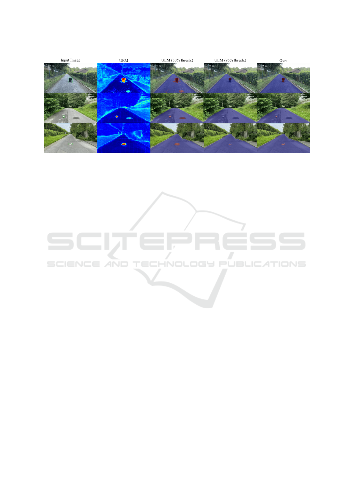
Figure 1: Road Obstacle Segmentation Overview. From the input image (anomaly highlighted with a green box), current

SOTA per-pixel methods (e.g., UEM (Nayal et al., 2024)) produce high anomaly scores for unknown objects (column two),

but when a threshold is applied the output is fragmented with multiple false positives or with false negatives if the threshold is

set too low or too high (column three and four). SAM produces high-quality segment masks for all image segments but lacks

semantic information. Our method (column ﬁve) uses the object priors used in SAM to learn the semantic distribution of the

segments and detect the road obstacle segments based on the likelihood ratios.

among classes, which is often the case for road ob-

stacles. However, they tend to be biased towards

larger obstacles, which is suboptimal as road obsta-

cles can vary substantially in size, and each is equally

important to detect. Component-level metrics are al-

ternative evaluation metrics that serve as an indirect

measure for object-level segmentation, assessing the

overlap between the predicted and actual regions of

anomalies. From a practitioner’s perspective, these

are the more interesting metrics to consider since

most downstream tasks would need detections and not

conﬁdence scores. Identifying the optimal threshold

is often a challenging and complex task. Setting the

threshold too low or too high can lead to either mul-

tiple false positives or missing detections (see Fig-

ure 1).

A common approach to threshold selection is to

analyze the pixel-level precision-recall curve and se-

lect the value that maximizes the F1 score on a per-

pixel basis. However, this approach requires a ded-

icated validation dataset and doesn’t always result

in optimal segment-level performance (Chan et al.,

2021). Furthermore, even with the optimal thresh-

old, the output masks produced by per-pixel detection

methods often need further reﬁnement, as some pix-

els may have inaccurate anomaly scores, resulting in

fragmented or discontinuous masks.

In this work, we utilize the strong object priors

in visual foundation models and present a method

for road obstacle detection using segment-level fea-

tures derived from the Segment Anything Model

(SAM) (Kirillov et al., 2023). Our approach gener-

ates more coherent and integrated segment-level pre-

dictions by focusing on segment features rather than

individual pixels, addressing the inherent limitations

of per-pixel predictions that often result in fragmented

predictions. The ﬁnal predictions are based on the

likelihood ratio of two learned distributions: free-

space and object segments. This allows us to miti-

gate the challenges associated with manual threshold

selection and improves the overall robustness of the

detection process.

In summary, we summarize our contributions as

follows:

• We introduce a novel road obstacle segmenta-

tion approach that leverages segment-level fea-

tures from visual foundational models, moving

beyond the pixel-level evaluation employed by ex-

isting methods.

• Our method utilizes a likelihood ratio between

learned distributions, eliminating the need for

manual threshold selection.

• We evaluate different approaches for learning the

free-space and obstacle segment distributions and

show that a non-parametric approach for approxi-

mating gives the best results.

• We demonstrate the effectiveness of our method

in generalizing to unseen road obstacles and com-

pare it to previous approaches on two bench-

marks, outperforming all other methods on

component-level metrics for both benchmarks.

Segment-Level Road Obstacle Detection Using Visual Foundation Model Priors and Likelihood Ratios

307

2 RELATED WORK

2.1 Road Obstacle Detection

Previous approaches for road obstacle detection relied

on multiple sensor modality setups to detect road ob-

stacles. (Williamson and Thorpe, 1998) used trinoc-

ular stereo vision and performed two types of stereo

matching to determine whether a pixel belongs to a

vertical or horizontal surface. (Pinggera et al., 2015)

used statistical hypothesis tests on local geometric

features captured from a stereo vision system to detect

obstacles. However, multi-camera systems present

additional challenges, such as requiring exact calibra-

tion to perform image wrapping and computing the

disparity between frames. In practice, vehicle vibra-

tion can complicate the calibration process since dif-

ferent cameras can move independently.

Other approaches required special types of sensors

like Light detection and ranging (LiDAR) or radio

detection and ranging (RADAR). (Tokudome et al.,

2017) used LiDAR sensors to measure the reﬂection

intensity of objects and detect road users. (Popov

et al., 2023) used RADAR signals for obstacle and

free space detection. While utilizing special sensor

modalities like LiDAR or RADAR signals could ben-

eﬁt obstacle detection, these specialized sensors are

not always available in all vehicle perception systems

due to costs and hardware limitations.

In this work, we focus only on methods that oper-

ate on single-frame images captured by standard in-

vehicle cameras as a promising alternative.

2.2 Road Obstacle Segmentation

The common approach for road obstacle segmen-

tation relies on a robust closed-world segmentation

model. This model is trained to detect a set of pre-

deﬁned classes and to quantify an OoD score for each

pixel that may belong to a different class. The per-

pixel OoD score can be interpreted as a form of pre-

dictive uncertainty on the given training set. Earlier

approaches modeled the uncertainty through maxi-

mum softmax probabilities (Hendrycks and Gimpel,

2017), ensembles (Lakshminarayanan et al., 2017),

Bayesian approximation (Mukhoti and Gal, 2018), or

Monte Carlo dropout (Gal and Ghahramani, 2016).

However, the posterior probabilities produced by a

model trained in a closed-word setting may not al-

ways be well-calibrated, often resulting in overly

conﬁdent predictions for unseen categories (Nguyen

et al., 2015b; Guo et al., 2017; Minderer et al., 2021;

Jiang et al., 2018). In this work, we utilize the strong

object priors that visual foundation models learn dur-

ing their training and utilize this to predict road obsta-

cles directly, without having a closed-world segmen-

tation model.

(Hendrycks et al., 2019a) introduced outlier expo-

sure as a strategy for enhancing the performance of

OoD detection. Outlier exposure leverages a proxy

dataset composed of outliers to discover signals and

learn heuristics for OoD samples. (Nayal et al., 2023)

used a proxy dataset to train the model to produce low

logit scores on unknown objects. We follow a similar

approach in our work, relying on a proxy dataset, but

we explicitly try to model the proxy distribution of

potential road obstacles and use this to differentiate

between free-space and obstacle segments.

2.3 Nearest-Neighbour OoD Detection

Retrieval-based methods have been explored for

anomaly detection (Reiss et al., 2021; Roth et al.,

2022; Zou et al., 2022), relying on large samples of

in-distribution datasets to identify anomalies as devi-

ations from the expected data patterns. (Sun et al.,

2022) highlighted the potential of using k-nearest-

neighbors (KNN) for OoD detection in deep neu-

ral networks. They used KNNs to calculate the dis-

tance between the embedding of each test image and

the training set, then applied a threshold-based cri-

terion to decide whether an input is OoD. However,

their exploration was limited to an image recognition

context, which is characterized by single-instance,

object-centric images. (Galesso et al., 2023) extended

the application of KNN to transformer-based repre-

sentations, achieving state-of-the-art performance on

common driving-focused anomaly detection bench-

marks. One limitation of their approach was its low

resolution, which limits its utility and applicability.

Our work adopts a similar strategy and uses KNNs to

learn feature representations from transformer-based

models. However, we learn two explicit distributions:

one for free-space and another for road obstacles.

This approach enhances the model’s ability to distin-

guish between road obstacles and road segments more

precisely.

2.4 Open-World Segmentation

Open-world segmentation seeks to segment all ob-

jects in the image, even those not in their training

dataset. Recent advancements in large-scale, text-

guided training for classiﬁcation (Jia et al., 2021;

Radford et al., 2021) have inspired several studies

to adapt and extend these methodologies to the do-

main of open-world segmentation (Rao et al., 2022;

Zheng Ding, 2023; Xu et al., 2022). However, a lim-

VISAPP 2025 - 20th International Conference on Computer Vision Theory and Applications

308

itation of these approaches is their reliance on text

prompts to segment objects. SEEM (Zou et al., 2023)

and Segment Anything Model (SAM) (Kirillov et al.,

2023) build upon previous work and allow for var-

ious types of prompts. In our approach, we leverage

SAM to generate and represent regions. Similar to our

work, (Nekrasov et al., 2023) also used SAM for road

obstacle detection, but they relied on an OoD seg-

mentation model to identify unknown regions and use

this to prompt SAM. In our approach, we directly use

SAM features to detect road obstacles which stream-

lines the process and potentially reduces reliance on

secondary models.

3 METHOD DESCRIPTION

We present our method in this section (see ﬁg. 2); we

ﬁrst give an overview of SAM and how we extract

segment-level feature representations. Next, we intro-

duce our task formulation for road obstacle detection,

focusing on how we leverage likelihood ratios to dif-

ferentiate between two learned distributions: one for

free-space segments and another for proxy road ob-

stacles. This approach allows us to detect road obsta-

cles more robustly by directly operating on segment-

level features, which mitigates the issues commonly

encountered with per-pixel predictions.

3.1 Preliminaries: Overview of SAM

SAM was recently introduced as a foundational vi-

sion model for general image segmentation. It was

trained on the large-scale SA-1B dataset, which con-

tains over 1 billion masks from 11 million images.

SAM’s architecture comprises three main modules: 1)

an image encoder for extracting image features, 2) a

prompt encoder that encodes positional information

from the input, and 3) a mask decoder that combines

the image features and prompt tokens to generate ﬁnal

mask predictions. Experimental results show power-

ful zero-shot capabilities to segment a wide range of

objects, parts, and visual structures across diverse sce-

narios. Therefore, an interesting question arises: can

we utilize SAM’s strong object priors for learning se-

mantic features of objects and regions?

However, efﬁciently extracting semantics from vi-

sual foundation models is a non-trivial challenge.

While a simple solution might be to use feature em-

beddings directly from the image encoder, we argue

that the prompt priors contained in the prompt tokens

are critical for accurately segmenting object bound-

aries. Therefore, we extract segment-level represen-

tations from the intermediate layers of the mask de-

coder, speciﬁcally after the transformer decoder lay-

ers and convolution (blue arrow in ﬁg. 2). Each

segment-level representation is a vector of size 2048,

encoding both the intersection over union prediction

and mask positions.

3.2 Road Obstacle Detection Using

Likelihood Ratios

A simple approach for road obstacle detection is to

learn a density model p

f ree

for free-space segments

and predict an obstacle when the likelihood p

f ree

(x)

of the input features x for is low (i.e., there is little

training data in the region around x ). However, since

we utilize neural networks that abstract information

and produce a condensed representation for each in-

put, utilizing only a single distribution for the task

may lead to unreliable results. As shown by (Nalis-

nick et al., 2019), a density estimate learned on one

dataset may assign higher scores to inputs from a

completely different dataset (i.e., one distribution may

sit inside of another distribution due to the feature ex-

traction process). This behavior suggests that using

a single distribution may fail to distinguish between

free-space and road obstacles effectively.

We formulate the road obstacle detection task as

a model selection task between two distributions rep-

resenting the free-space segments P

f ree

and obstacles

obstacle

. Given a feature vector x, consider the null

hypothesis H

f ree

that x was drawn from P

f ree

, and an

alternate hypothesis H

obstacle

that x was drawn from

obstacle

. By the Neyman-Pearson lemma (Neyman

and Pearson, 1933), when ﬁxing type-I errors (false-

positives), the test with the smallest type-II errors

(false-negatives) is the likelihood ratio test.

LR =

obstacle

(x)

f ree

(x)

(1)

(Zhang and Wischik, 2022) showed that the same

conclusion holds for a Bayesian perspective. Di-

rectly predicting the ﬁnal output from this ratio is a

formulation of the Maximum Likelihood (ML) deci-

sion rule (Fahrmeir et al., 1996) from decision the-

ory. Since road obstacles are very rare in practice,

this would mean that the ML would overestimate the

likelihood of road obstacles. However, from a safety

perspective, basing the detections only on the most

likely observed features would be more desirable than

potentially biasing our decision based on prior knowl-

edge.

While it is infeasible to estimate the true distribu-

tion P

obstacle

for every potential road obstacle—given

the wide variability in obstacle types—we adopt the

concept of outlier exposure (Hendrycks et al., 2019b)

Segment-Level Road Obstacle Detection Using Visual Foundation Model Priors and Likelihood Ratios

309

Input Image

Image

Encoder

Prompt

Decoder

Decoder Layer

Transposed

Conv

Token

Attention

Mask Decoder

Segment-level

Features

Likelihood

Ratios

Binary

Predictions

Road-Distribution

Obstacle-Distribution

Segment

Masks

Figure 2: Approach For Segment-Level Road Obstacle Detection: Our approach for road obstacle detection uses visual

foundation models like SAM (Kirillov et al., 2023) to generate segment-level masks. The segment-level feature representa-

tions are obtained from the transformer decoder layer, which processes the image and prompts embeddings. During inference,

we generate masks for the entire image using a grid of point prompts over the image and ﬁlter low-quality and duplicate masks

outside the region of interest. For each remaining mask, we compute the likelihood ratios of these learned representations to

produce ﬁnal predictions using two learned estimates trained to estimate free space and obstacles.

to approximate P

obstacle

using a proxy dataset. This

proxy dataset captures a diverse set of possible ob-

stacles, allowing us to model the distribution without

accounting for every scenario. Importantly, in our for-

mulation, the obstacle distribution does not need to

be perfectly precise. Rather, it only needs to exhibit

greater similarity to the proxy dataset than to the dis-

tribution of free-space segments, making it sufﬁcient

for effective obstacle detection.

3.3 Distribution Estimation Methods

We build two reference feature datasets for the free-

space segments and out-distribution datasets. Both

datasets are obtained from an internal dataset that

contains labeled road obstacles captured from a real-

world test vehicle in both urban and highway driving

conditions. The reference feature datasets are denoted

as R

f ree

∈ R

N×C

and R

obstacle

∈ R

M×C

where N and

M are the number of reference features and C is the

dimensionality of each reference features. For both

datasets, the dimensionality C is 2048, and the num-

ber of reference features is 10k. We evaluate three

distinct approaches for estimating the distributions of

these datasets: Gaussian Mixture Models (GMMs),

which provide log-likelihood estimates; Normalizing

Flows, which offer exact density estimates; and k-

Nearest Neighbours (k-NN), which compute odds es-

timates based on neighborhood distances of the fea-

ture representations. We dive into the details of each

method in this section.

3.3.1 Gaussian Mixture Models

Gaussian Mixture Models (GMMs) assume that the

feature vectors in a dataset are generated from a mix-

ture of several Gaussian distributions. Each Gaussian

distribution in the mixture represents a different clus-

ter, characterized by its own mean vector and covari-

ance matrix. Formally, the probability density func-

tion of a GMM is expressed as:

p(x | λ) =

∑

i=1

N (x | µ

,Σ

)

where K is the number of Gaussian compo-

nents, π

represents the mixing coefﬁcients (such that

∑

i=1

= 1), µ

is the mean, and Σ

is the covariance

matrix of the i-th component.

We ﬁt two separate GMMs, on R

and on R

out

to model the in-distribution and out-distribution fea-

ture sets, respectively. The GMM parameters λ

{π

,µ

,Σ

} are estimated from R

, while the pa-

rameters λ

out

= {π

out

,µ

out

,Σ

out

} are estimated from

out

During inference, we compute the likelihood

of each segment-level feature t under both the in-

distribution and out-distribution models. This is done

by calculating the likelihood of t under each GMM:

VISAPP 2025 - 20th International Conference on Computer Vision Theory and Applications

310

p(t | λ

) =

∑

i=1

N (t | µ

,Σ

)

p(t | λ

out

) =

∑

i=1

out

N (t | µ

out

,Σ

out

)

We then compare the odds estimate of both dis-

tributions. If p(t | λ

)/p(t | λ

out

) ≥ 1, we predict

that the test sample t belongs to the in-distribution.

Otherwise, we classify it as belonging to the out-

distribution.

We use a GMM with K = 50 components and

a diagonal covariance matrix, which balances model

complexity and accuracy in distinguishing between

in-distribution and out-distribution samples. The

parameters of the GMM are estimated using the

Maximum Likelihood estimator for the observed

data using the Expectation Maximization (EM) algo-

rithm (Dempster et al., 1977) with initialization done

using K-means clustering.

3.3.2 Normalizing Flows

Normalizing Flows (NF) are a class of generative

models that use a sequence of invertible transforma-

tions to map a simple prior distribution (e.g., Gaus-

sian) to a more complex distribution that ﬁts the data.

Each transformation in the ﬂow is designed to be both

invertible and differentiable, allowing for the com-

putation of both the density and sampling (Kobyzev

et al., 2021). We learn a ﬂow for each distribution and

use the density estimates to predict which distribution

the sample belongs to.

In our approach, we use Neural Spline

Flows (Durkan et al., 2019), speciﬁcally cou-

pling layers based on rational quadratic splines. The

splines parameterize piecewise invertible functions,

making mapping between simple and complex

distributions possible. The transformations are

conditioned on half of the input dimensions, which

are learned via a four-layer MLP.

The overall ﬂow is constructed by a sequence

of three blocks, where each block includes an act-

norm layer, an Invertible 1x1 Convolution (Hooge-

boom et al., 2019), and a Neural Spline Flow. The

ﬂow is designed to map the input data distribution

to a standard Gaussian prior N (0,1). During infer-

ence, each segment-level feature t is passed through

the model transforms, and the log probability score

is computed for each model approximating the free-

space and road obstacle. If the log probability scores

for road obstacle model is larger than the log proba-

bility scores for the free-space model, then we predict

the segment to be an obstacle.

3.3.3 K-Nearest Neighbors

k-Nearest Neighbors relies on the computation of dis-

tances between feature representations as a measure

of estimation. More formally, each segment-level

feature t of the image is extracted, and the distance

to each of the features in R

and R

out

denoted as

dist(t,x

) and dist(t, x

out

). We then ﬁnd the k sam-

ples with the highest cosine similarity values to t in

and R

out

. Let N

(t) and N

out

(t) be the sets of

the top-k most similar samples to t based on the co-

sine similarity values. The average cosine similarity

between t and the top-k most similar samples in R are

calculated as:

dist(t,N

(t)) =

∑

∈N

(t)

dist(t,x

) (2)

dist(t,N

obstacle

(t))

dist(t,N

f ree

(t))

≥ 1 we predict that the test sample

t is more likely to be an obstacle. We use the cosine

similarity as a distance metric and ﬁnd k equal to ﬁve

to give the best results.

4 EXPERIMENTS

4.1 Experimental Setup

Metrics. The standard metrics for pixel-level seg-

mentation are Average Precision (AP) and False Pos-

itive Rate at a True Positive Rate of 95% (FPR95).

These are all threshold-independent metrics, which

help evaluate the usability of a method irrespective

of the chosen threshold. However, in practice, a

threshold must always be selected for any down-

stream task that utilizes an OoD detector (Maag et al.,

2022; Shoeb et al., 2024). Therefore, we focus on

the three component-level metrics used in the Seg-

mentMeIfYouCan (SMIYC) benchmark (Chan et al.,

2021) (sIoU

, PPV, and mean F

) as our main com-

parison metric. sIoU

is the average intersection over

union, measuring how well the prediction road obsta-

cle overlaps with the ground truth. PPV is the average

positive predictive value, and this asses how accurate

the predicted road obstacles are (precision). Finally,

mean F

is a balanced measure combining both sIoU

and PPV. It is calculated at multiple thresholds and

then averaged; this provides a single value reﬂecting

both the ability to detect and the accuracy of these de-

tections.

Datasets. We evaluate our method on SMIYC-

RoadObstacle, and SMIYC-LostAndFound. Both

datasets represent realistic and hazardous obstacles

Segment-Level Road Obstacle Detection Using Visual Foundation Model Priors and Likelihood Ratios

311

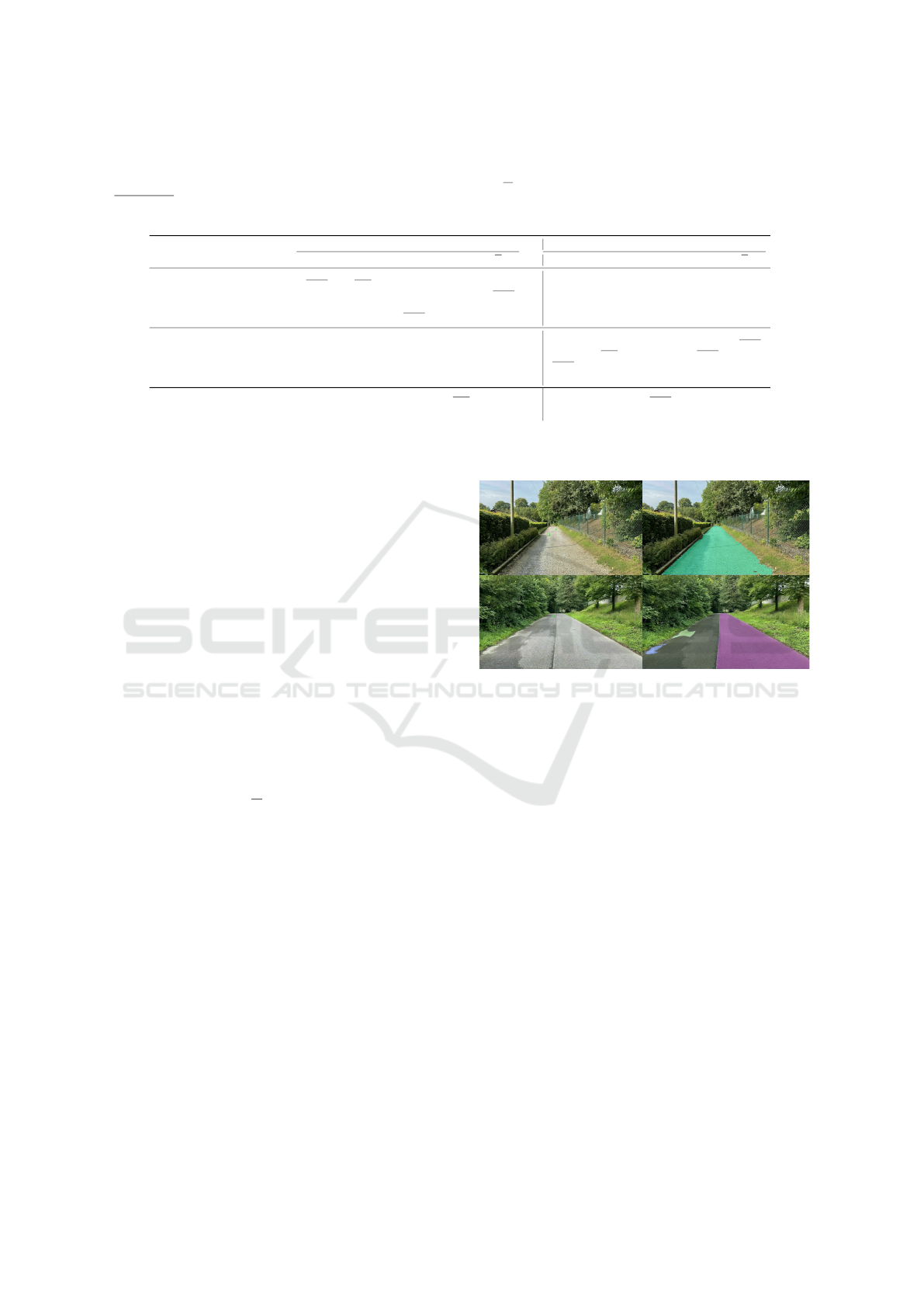
Table 1: Performance on SMIYC-Obstacle and SMIYC-LostAndFound Benchmarks: We compare the performance of

the top-ﬁve state-of-the-art methods across both datasets. The best results are highlighted in bold, and the second best are

underlined. Our method achieves state-of-the-art performance on the F1 score and PPV in the component-level metrics. On

pixel-level metrics, our method is not as competitive as state-of-the-art pixel segmentation networks due to obstacles that are

missed and assigned as a road by default.

Method

SMIYC-Obstacle SMIYC-LostAndFound

AP ↑ FPR

↓ sIoU

↑ PPV ↑ F

↑ AP ↑ FPR

↓ sIoU

↑ PPV ↑ F

↑

UEM (Nayal et al., 2024) 94.40 0.10 49.80 76.80 67.2

UNO (Deli

c et al., 2024) 93.19 0.16 70.97 72.17 77.65

RbA (Nayal et al., 2023) 95.12 0.08 54.34 59.08 57.44

EAM (Grci

c et al., 2023) 92.87 0.52 65.86 76.50 75.58

Mask2Anomaly (Rai et al., 2023) 93.22 0.20 55.72 75.42 68.15

NFlowJS (Grci

c et al., 2023) 89.28 0.65 54.63 59.74 61.75

PixOOD (Voj

r et al., 2024) 85.07 4.46 30.18 78.47 44.41

Road Inpainting (Lis et al., 2023) 82.93 35.75 49.21 60.67 52.25

SynBoost (Di Biase et al., 2021) 81.71 4.64 36.83 72.32 48.72

DaCUP (Voj

r and Matas, 2023) 81.37 7.36 38.34 67.29 51.14

LR (KNN) -ours- 92.0 0.20 62.9 81.9 78.4 83.70 - 49.70 95.90 72.60

LR (GMM) -ours- 91.90 0.20 59.5 84.2 76.90 83.50 - 47.40 92.00 69.20

LR (NF) -ours- 77.10 33.70 46.50 77.5 62.70 76.90 - 44.70 73.50 61.00

on the road ahead that are critical to detect for

an autonomous vehicle. SMIYC-RoadObstacle con-

tains a total of 327 privately withheld images, which

are used to evaluate different methods. SMIYC-

LostAndFound is a ﬁltered and reﬁned- version of Lo-

stAndFound (Pinggera et al., 2016).

4.2 Comparison to State-of-the-Art

We evaluate our proposed method with different dis-

tribution estimation methods, as shown in Table 1.

Each approach is compared against the top ﬁve

state-of-the-art methods on the SMIYC-Obstacle and

SMIYC-LostAndFound datasets. Our results demon-

strate that our method achieves competitive perfor-

mance across all three distribution estimation tech-

niques, with the non-parametric k-nearest neighbor

approach yielding the best results on both datasets.

The most signiﬁcant improvement is observed on

SMIYC-LostAndFound, where our method achieves

a PPV of 95.9 and an F

score of 72.60, outperform-

ing the previous best method by 17.43 and 10.85, re-

spectively.

However, in pixel-level metrics such as aver-

age precision (AP) and false positive rate (FPR),

our method is less competitive compared to state-

of-the-art pixel segmentation networks like RbA and

NFlowJS. This discrepancy can be attributed to the

limitations of our model in detecting smaller or am-

biguous obstacles, which are sometimes not detected

as separate segments by SAM as seen in Figure 3.

Additionally, this causes the FPR

metric to fail on

the SMIYC-LostAndFound dataset as more than 5%

of the obstacles are not detected as separate segments

and are considered free space by default. Despite this,

the superior performance in component-level metrics

suggests that our method is highly effective at distin-

guishing between larger and more well-deﬁned obsta-

cles, which is critical for real-world applications of

road obstacle detection.

Figure 3: Failure Case Examples: The left column shows

the input image with the road obstacles highlighted in green

bounding boxes, and the right column shows scenarios

where the masks generated by SAM miss detecting the road

obstacle as a separate segment.

4.3 Ablations

For each estimation method, we visualize the sepa-

ration between the two learned distributions on the

training data in Figure 4. The ﬁrst row visualizes the

likelihood of sampling from each GMM, the second

row visualizes the density estimates for each normal-

izing ﬂow model, and the ﬁnal row visualizes one mi-

nus the average distance to the 5 nearest neighbors.

For all three methods, utilizing the likelihood ratio

between the two distributions provides a better sep-

aration than utilizing any one model on its own. We

also ﬁnd that the normalizing ﬂow models provide the

best separation of the training data. However, it does

not generalize as well as the GMM or the k-nearest

neighbors.

VISAPP 2025 - 20th International Conference on Computer Vision Theory and Applications

312

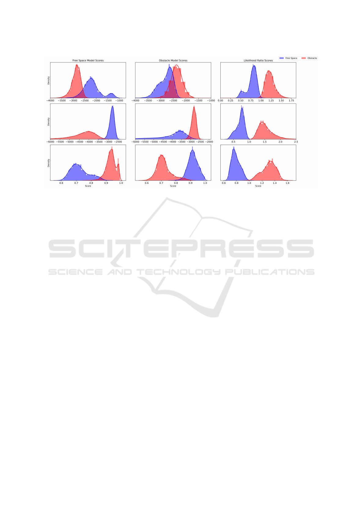
Figure 4: Comparison of Gaussian Mixture Models (ﬁrst row) Normalizing Flows (second row), and K-nearest neighbors

(third row) on the training set. The ﬁrst column visualizes the learned distributions of the free-space model, the second

visualizes the learned distributions of obstacles, and the third visualizes the likelihood ratio between both. The likelihood

ratio provides better separation than any of the models separately at the threshold value 1.

5 CONCLUSION & OUTLOOK

In this paper, we propose a novel approach to address

the road obstacle segmentation problem at the seg-

ment level. Our method leverages strong object priors

from visual foundational models to generate segment-

level features. We estimate the probability distribu-

tions for both free-space and obstacle segments and

utilize the likelihood ratios as a binary classiﬁer to

detect road obstacles. We evaluate several methods

for estimating these distributions, including GMMs,

normalizing ﬂows, and k-nearest neighbors, ﬁnding

that k-nearest neighbors produce the best results.

Our approach achieves state-of-the-art performance

on standard benchmarks (SegmentMeIfYouCan and

LostAndFound) in terms of component-level metrics

without requiring a predeﬁned threshold. Limita-

tions and Future Work: Despite the strong perfor-

mance in component-level metrics, our approach still

suffers from a relatively high false-negative rate due

to small objects not being detected as separate seg-

ments by SAM. This is due to the prompting strategy

we deploy; the equally spaced grid may miss small

objects that lie between the point prompts. Restricting

the prompts to only regions where the model is uncer-

tain could potentially resolve this issue, but then the

segments that the model incorrectly classiﬁes as the

road will also be missed from the road obstacle de-

tection module. Additionally, the efﬁcacy of the best-

performing method (k-nearest neighbours) relies on

the number and quality of reference features selected.

In this work, we utilized all available reference fea-

tures without examining the impact of selecting dif-

ferent subsets of these features. Future work would

investigate the application of more sophisticated tech-

niques, such as core-set approaches (Tereshchenko

and Zakala, 2024), to choose the set of reference fea-

tures selectively. By optimizing the selection process,

we anticipated that the inference time of our models

could be signiﬁcantly enhanced without loss in per-

formance.

ACKNOWLEDGEMENTS

The research leading to these results is funded by the

German Federal Ministry for Economic Affairs and

Climate Action within the project “just better DATA”.

N.N. is funded by the KUIS AI Center, F.G. by the Eu-

ropean Union (ERC, ENSURE, 101116486). Views

and opinions expressed are however those of the au-

thor(s) only and do not necessarily reﬂect those of the

European Union or the European Research Council.

Neither the European Union nor the granting author-

ity can be held responsible for them.

Segment-Level Road Obstacle Detection Using Visual Foundation Model Priors and Likelihood Ratios

313

REFERENCES

Ackermann, J., Sakaridis, C., and Yu, F. (2023). Masko-

maly: Zero-shot mask anomaly segmentation. In The

British Machine Vision Conference (BMVC).

Chan, R., Lis, K., Uhlemeyer, S., Blum, H., Honari, S.,

Siegwart, R., Fua, P., Salzmann, M., and Rottmann,

M. (2021). Segmentmeifyoucan: A benchmark for

anomaly segmentation. In Thirty-ﬁfth Conference on

Neural Information Processing Systems Datasets and

Benchmarks Track.

Deli

c, A., Grci

c, M., and

Segvi

c, S. (2024). Outlier detec-

tion by ensembling uncertainty with negative object-

ness.

Dempster, A. P., Laird, N. M., and Rubin, D. B. (1977).

Maximum likelihood from incomplete data via the em

algorithm. Journal of the royal statistical society: se-

ries B (methodological), 39(1):1–22.

Di Biase, G., Blum, H., Siegwart, R., and Cadena, C.

(2021). Pixel-wise anomaly detection in complex

driving scenes. In 2021 IEEE/CVF Conference on

Computer Vision and Pattern Recognition (CVPR),

pages 16913–16922.

Durkan, C., Bekasov, A., Murray, I., and Papamakarios,

G. (2019). Neural spline ﬂows. In Wallach, H.,

Larochelle, H., Beygelzimer, A., d'Alch

e-Buc, F.,

Fox, E., and Garnett, R., editors, Advances in Neural

Information Processing Systems, volume 32. Curran

Associates, Inc.

Fahrmeir, L., Hamerle, A., and Tutz, G., editors (1996).

Multivariate statistische Verfahren. De Gruyter,

Berlin, Boston.

Gal, Y. and Ghahramani, Z. (2016). Dropout as a bayesian

approximation: Representing model uncertainty in

deep learning. In ICML.

Galesso, S., Argus, M., and Brox, T. (2023). Far away

in the deep space: Dense nearest-neighbor-based out-

of-distribution detection. In 2023 IEEE/CVF In-

ternational Conference on Computer Vision Work-

shops (ICCVW), pages 4479–4489, Los Alamitos,

CA, USA. IEEE Computer Society.

Grci

c, M.,

Sari

c, J., and

Segvi

c, S. (2023). On advantages

of mask-level recognition for outlier-aware segmenta-

tion. In CVPR Workshops.

Grci

c, M., Bevandi

c, P., Kalafati

c, Z., and

Segvi

c, S.

(2023). Dense out-of-distribution detection by robust

learning on synthetic negative data.

Guo, C., Pleiss, G., Sun, Y., and Weinberger, K. Q. (2017).

On calibration of modern neural networks. In ICML.

Hendrycks, D. and Gimpel, K. (2017). A baseline for de-

tecting misclassiﬁed and out-of-distribution examples

in neural networks. In ICLR.

Hendrycks, D., Mazeika, M., and Dietterich, T. (2019a).

Deep anomaly detection with outlier exposure. Pro-

ceedings of the International Conference on Learning

Representations.

Hendrycks, D., Mazeika, M., and Dietterich, T. (2019b).

Deep anomaly detection with outlier exposure. In

ICLR.

Hoogeboom, E., Van Den Berg, R., and Welling, M.

(2019). Emerging convolutions for generative nor-

malizing ﬂows. In Chaudhuri, K. and Salakhutdi-

nov, R., editors, Proceedings of the 36th International

Conference on Machine Learning, volume 97 of Pro-

ceedings of Machine Learning Research, pages 2771–

2780. PMLR.

Jia, C., Yang, Y., Xia, Y., Chen, Y.-T., Parekh, Z., Pham,

H., Le, Q., Sung, Y.-H., Li, Z., and Duerig, T. (2021).

Scaling up visual and vision-language representation

learning with noisy text supervision. In Meila, M. and

Zhang, T., editors, Proceedings of the 38th Interna-

tional Conference on Machine Learning, volume 139

of Proceedings of Machine Learning Research, pages

4904–4916. PMLR.

Jiang, H., Kim, B., Guan, M., and Gupta, M. (2018). To

trust or not to trust a classiﬁer. In NeurIPS.

Kirillov, A., Mintun, E., Ravi, N., Mao, H., Rolland, C.,

Gustafson, L., Xiao, T., Whitehead, S., Berg, A. C.,

Lo, W.-Y., Dollar, P., and Girshick, R. (2023). Seg-

ment anything. In Proceedings of the IEEE/CVF In-

ternational Conference on Computer Vision (ICCV),

pages 4015–4026.

Kobyzev, I., Prince, S. J., and Brubaker, M. A. (2021). Nor-

malizing ﬂows: An introduction and review of current

methods. IEEE Transactions on Pattern Analysis and

Machine Intelligence, 43(11):3964–3979.

Lakshminarayanan, B., Pritzel, A., and Blundell, C. (2017).

Simple and scalable predictive uncertainty estimation

using deep ensembles. In NeurIPS.

Lis, K., Honari, S., Fua, P., and Salzmann, M. (2023). De-

tecting road obstacles by erasing them. IEEE Trans-

actions on Pattern Analysis and Machine Intelligence,

pages 1–11.

Maag, K., Chan, R., Uhlemeyer, S., Kowol, K., and

Gottschalk, H. (2022). Two video data sets for track-

ing and retrieval of out of distribution objects. In Pro-

ceedings of the Asian Conference on Computer Vision,

pages 3776–3794.

Minderer, M., Djolonga, J., Romijnders, R., Hubis, F. A.,

Zhai, X., Houlsby, N., Tran, D., and Lucic, M. (2021).

Revisiting the calibration of modern neural networks.

In NeurIPS.

Mukhoti, J. and Gal, Y. (2018). Evaluating bayesian

deep learning methods for semantic segmentation.

1811.12709.

Nalisnick, E., Matsukawa, A., Teh, Y. W., Gorur, D., and

Lakshminarayanan, B. (2019). Do deep generative

models know what they don’t know? International

Conference on Learning Representations.

Nayal, N., Shoeb, Y., and G

uney, F. (2024). A likelihood

ratio-based approach to segmenting unknown objects.

Nayal, N., Yavuz, M., Henriques, J. F., and G

uney, F.

(2023). Rba: Segmenting unknown regions rejected

by all. In ICCV.

Nekrasov, A., Hermans, A., Kuhnert, L., and Leibe, B.

(2023). UGainS: Uncertainty Guided Anomaly In-

stance Segmentation. In GCPR.

Neyman, J. and Pearson, E. S. (1933). Ix. on the problem of

the most efﬁcient tests of statistical hypotheses. Philo-

VISAPP 2025 - 20th International Conference on Computer Vision Theory and Applications

314

sophical Transactions of the Royal Society of Lon-

don. Series A, Containing Papers of a Mathematical

or Physical Character, 231(694-706):289–337.

Nguyen, A., Yosinski, J., and Clune, J. (2015a). Deep neu-

ral networks are easily fooled: High conﬁdence pre-

dictions for unrecognizable images. In CVPR, pages

427–436.

Nguyen, A. M., Yosinski, J., and Clune, J. (2015b). Deep

neural networks are easily fooled: High conﬁdence

predictions for unrecognizable images. In CVPR.

Pinggera, P., Franke, U., and Mester, R. (2015). High-

performance long range obstacle detection using

stereo vision. In 2015 IEEE/RSJ International Confer-

ence on Intelligent Robots and Systems (IROS), pages

1308–1313.

Pinggera, P., Ramos, S., Gehrig, S., Franke, U., Rother,

C., and Mester, R. (2016). Lost and found: detect-

ing small road hazards for self-driving vehicles. In

2016 IEEE/RSJ International Conference on Intelli-

gent Robots and Systems (IROS), page 1099–1106.

IEEE Press.

Popov, A., Gebhardt, P., Chen, K., and Oldja, R. (2023).

Nvradarnet: Real-time radar obstacle and free space

detection for autonomous driving. In 2023 IEEE In-

ternational Conference on Robotics and Automation

(ICRA), pages 6958–6964.

Radford, A., Kim, J. W., Hallacy, C., Ramesh, A., Goh,

G., Agarwal, S., Sastry, G., Askell, A., Mishkin, P.,

Clark, J., Krueger, G., and Sutskever, I. (2021). Learn-

ing transferable visual models from natural language

supervision. In Meila, M. and Zhang, T., editors, Pro-

ceedings of the 38th International Conference on Ma-

chine Learning, volume 139 of Proceedings of Ma-

chine Learning Research, pages 8748–8763. PMLR.

Rai, S. N., Cermelli, F., Fontanel, D., Masone, C., and Ca-

puto, B. (2023). Unmasking anomalies in road-scene

segmentation. In Proceedings of the IEEE/CVF In-

ternational Conference on Computer Vision (ICCV),

pages 4037–4046.

Rao, Y., Zhao, W., Chen, G., Tang, Y., Zhu, Z., Huang, G.,

Zhou, J., and Lu, J. (2022). Denseclip: Language-

guided dense prediction with context-aware prompt-

ing. In Proceedings of the IEEE Conference on Com-

puter Vision and Pattern Recognition (CVPR).

Reiss, T., Cohen, N., Bergman, L., and Hoshen, Y. (2021).

Panda: Adapting pretrained features for anomaly de-

tection and segmentation. In Proceedings of the

IEEE/CVF Conference on Computer Vision and Pat-

tern Recognition, pages 2806–2814.

Roth, K., Pemula, L., Zepeda, J., Sch

olkopf, B., Brox, T.,

and Gehler, P. (2022). Towards total recall in in-

dustrial anomaly detection. In 2022 IEEE/CVF Con-

ference on Computer Vision and Pattern Recognition

(CVPR), pages 14298–14308.

Shoeb, Y., Chan, R., Schwalbe, G., Nowzad, A., G

uney,

F., and Gottschalk, H. (2024). Have we ever en-

countered this before? retrieving out-of-distribution

road obstacles from driving scenes. In Proceedings of

the IEEE/CVF Winter Conference on Applications of

Computer Vision, pages 7396–7406.

Sun, Y., Ming, Y., Zhu, X., and Li, Y. (2022). Out-

of-distribution detection with deep nearest neighbors.

ICML.

Tereshchenko, V. and Zakala, P. (2024). Coreset discov-

ery for machine learning problems. Cybernetics and

Systems Analysis, 60:198–208.

Tian, Y., Liu, Y., Pang, G., Liu, F., Chen, Y., and Carneiro,

G. (2022). Pixel-wise energy-biased abstention learn-

ing for anomaly segmentation on complex urban driv-

ing scenes. In Avidan, S., Brostow, G., Ciss

e, M.,

Farinella, G. M., and Hassner, T., editors, Computer

Vision – ECCV 2022, pages 246–263, Cham. Springer

Nature Switzerland.

Tokudome, N., Ayukawa, S., Ninomiya, S., Enokida, S.,

and Nishida, T. (2017). Development of real-time

environment recognition system using lidar for au-

tonomous driving. In International Conference on ICT

Robotics, volume 2017, pages 25–26.

Voj

r, T. and Matas, J. (2023). Image-consistent detection of

road anomalies as unpredictable patches. In Proceed-

ings of the IEEE/CVF Winter Conference on Applica-

tions of Computer Vision (WACV), pages 5491–5500.

Voj

r, T.,

Sochman, J., and Matas, J. (2024). PixOOD:

Pixel-Level Out-of-Distribution Detection. In ECCV.

Williamson, T. and Thorpe, C. E. (1998). Detection of small

obstacles at long range using multibaseline stereo.

Xu, J., De Mello, S., Liu, S., Byeon, W., Breuel, T., Kautz,

J., and Wang, X. (2022). Groupvit: Semantic seg-

mentation emerges from text supervision. In 2022

IEEE/CVF Conference on Computer Vision and Pat-

tern Recognition (CVPR), pages 18113–18123.

Zhang, A. and Wischik, D. (2022). Falsehoods that ml re-

searchers believe about ood detection. In NeurIPS ML

Safety Workshop.

Zheng Ding, Jieke Wang, Z. T. (2023). Open-vocabulary

universal image segmentation with maskclip. In In-

ternational Conference on Machine Learning.

Zou, X., Yang, J., Zhang, H., Li, F., Li, L., Wang, J., Wang,

L., Gao, J., and Lee, Y. J. (2023). Segment everything

everywhere all at once. In Advances in Neural Infor-

mation Processing Systems.

Zou, Y., Jeong, J., Pemula, L., Zhang, D., and Dabeer,

O. (2022). Spot-the-difference self-supervised pre-

training for anomaly detection and segmentation.

In Avidan, S., Brostow, G., Ciss

e, M., Farinella,

G. M., and Hassner, T., editors, Computer Vision –

ECCV 2022, pages 392–408, Cham. Springer Nature

Switzerland.

Segment-Level Road Obstacle Detection Using Visual Foundation Model Priors and Likelihood Ratios

315