Classifier Ensemble for Efficient Uncertainty Calibration of Deep Neural
Networks for Image Classification
Michael Schulze, Nikolas Ebert, Laurenz Reichardt and Oliver Wasenm
¨
uller
Mannheim University of Applied Sciences, Germany
Keywords:
Calibration, Uncertainty, Image Classification, SafeAI, XAI.
Abstract:
This paper investigates novel classifier ensemble techniques for uncertainty calibration applied to various deep
neural networks for image classification. We evaluate both accuracy and calibration metrics, focusing on Ex-
pected Calibration Error (ECE) and Maximum Calibration Error (MCE). Our work compares different meth-
ods for building simple yet efficient classifier ensembles, including majority voting and several metamodel-
based approaches. Our evaluation reveals that while state-of-the-art deep neural networks for image classifi-
cation achieve high accuracy on standard datasets, they frequently suffer from significant calibration errors.
Basic ensemble techniques like majority voting provide modest improvements, while metamodel-based en-
sembles consistently reduce ECE and MCE across all architectures. Notably, the largest of our compared
metamodels demonstrate the most substantial calibration improvements, with minimal impact on accuracy.
Moreover, classifier ensembles with metamodels outperform traditional model ensembles in calibration per-
formance, while requiring significantly fewer parameters. In comparison to traditional post-hoc calibration
methods, our approach removes the need for a separate calibration dataset. These findings underscore the
potential of our proposed metamodel-based classifier ensembles as an efficient and effective approach to im-
proving model calibration, thereby contributing to more reliable deep learning systems.
1 INTRODUCTION
Machine learning models, particularly deep neural
networks, are increasingly applied in safety critical
areas such as autonomous driving (Ebert et al., 2022;
Reichardt et al., 2023) and medical image analysis
(Ebert et al., 2023), where incorrect decisions can
have serious consequences. In these settings, achiev-
ing high accuracy and robustness (Oehri et al., 2024;
Kendall and Gal, 2017) is crucial, but models must
also provide reliable uncertainty estimates to assess
whether their predictions can be trusted (Jiang et al.,
2018). Calibration addresses this need by align-
ing predicted probabilities with the true likelihood
of predictions being correct (Br
¨
ocker, 2009). How-
ever many machine learning models (Niculescu-Mizil
and Caruana, 2005), especially deep neural networks
(Guo et al., 2017), are poorly calibrated and tend to
produce overconfident predictions, even when they
are wrong.
Post-hoc calibration methods, which adjust the
prediction scores of a trained neural network us-
ing a separate calibration dataset, are widely used
to improve uncertainty estimates. Examples in-
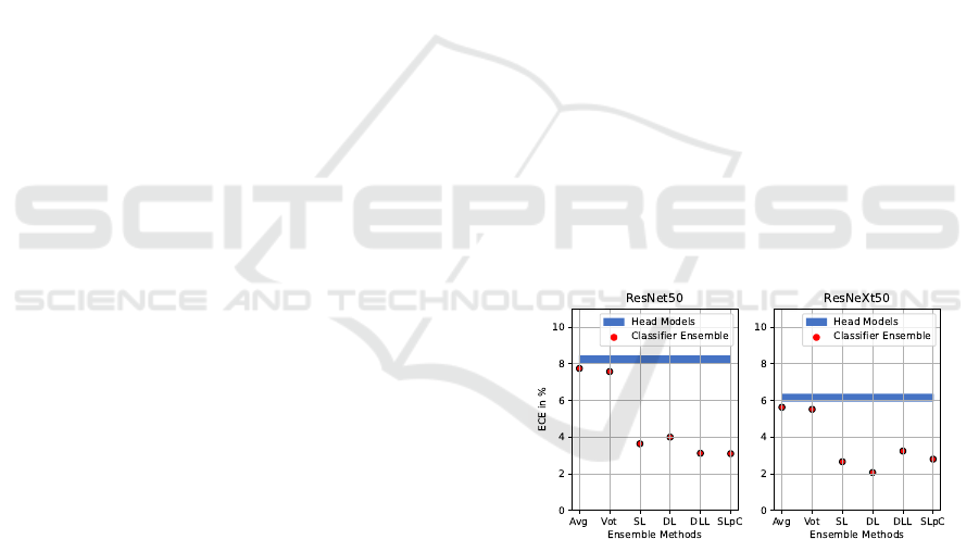
Figure 1: Expected Calibration Error (ECE) of ResNet50
(He et al., 2016) (left) and ResNeXt50 (Xie et al., 2017)
(right) on CIFAR-100 (Krizhevsky et al., 2009). Each
model was trained with five classifier heads initialized with
different random seeds but using the same backbone. The
blue area represents the ECE range for the uncalibrated clas-
sifiers. Each red dot corresponds to the ECE value achieved
using different ensemble techniques. The use of metamod-
els (SL, DL, DLL, SLpC) significantly improves the cali-
bration performance and reduces the ECE compared to the
uncalibrated baseline.
clude Platt scaling (Platt et al., 1999), histogram bin-
ning (Zadrozny and Elkan, 2001), isotonic regression
(Zadrozny and Elkan, 2002) and temperature scaling
316
Schulze, M., Ebert, N., Reichardt, L. and Wasenmüller, O.
Classifier Ensemble for Efficient Uncertainty Calibration of Deep Neural Networks for Image Classification.
DOI: 10.5220/0013129000003912
Paper published under CC license (CC BY-NC-ND 4.0)
In Proceedings of the 20th International Joint Conference on Computer Vision, Imaging and Computer Graphics Theory and Applications (VISIGRAPP 2025) - Volume 2: VISAPP, pages
316-323
ISBN: 978-989-758-728-3; ISSN: 2184-4321
Proceedings Copyright © 2025 by SCITEPRESS – Science and Technology Publications, Lda.

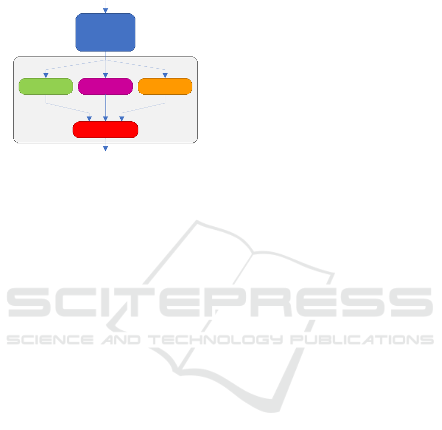
Backbone
Head 1 ... Head m
Combination
Figure 2: The principle of the classifier ensemble involves a
single backbone that feeds multiple classifiers (heads). The
combination method can be freely selected.
(Guo et al., 2017). Parametric methods like tempera-
ture scaling rescale the output logits of a neural net-
work for classification using learned parameters from
a calibration set. However, in many real-world scenar-
ios with limited data, a dedicated calibration set is not
available. Although non-parametric methods, such as
isotonic regression, offer greater flexibility, they can
reduce model accuracy after calibration. Similar to
their parametric counterparts, these methods also re-
quire a dedicated calibration set.
In contrast to post-hoc calibration, ab-initio meth-
ods (Lakshminarayanan et al., 2017; Kumar et al.,
2018) aim to train models that are well-calibrated
from the start, incorporating uncertainty directly dur-
ing training. Furthermore, deep ensembles (Lakshmi-
narayanan et al., 2017; Wenzel et al., 2020) combine
multiple models trained on the same dataset through
majority voting or averaging, which enhances accu-
racy and reduces uncertainty. However, a disadvan-
tage of this approach is the high computational cost
associated with training several independent models.
In contrast, Monte Carlo dropout (Gal and Ghahra-
mani, 2016) follows a similar strategy by applying
dropout during training and inference to randomly de-
activate individual neurons, thereby creating an en-
semble of models. However, this method requires
repeated inference, resulting in lower accuracy and
higher uncertainty compared to deep ensembles.
Thus, we propose a novel approach based on clas-
sifier ensemble (see Figure 2), which effectively com-
bines transfer learning with ensemble methods for ef-
ficient uncertainty calibration. In contrast to tradi-
tional ensemble techniques, where multiple full-scale
networks are trained separately and their predictions
are combined, our method focuses on training mul-
tiple lightweight classifiers on-top of a shared back-
bone and utilizing their predictions collaboratively.
This technique stands out by eliminating the need for
an additional calibration dataset and significantly re-
ducing computational overhead during both training
and inference. By combining the strengths of transfer
learning and ensemble methods, our classifier ensem-
ble significantly reduces uncertainty while maintain-
ing computational efficiency. Furthermore, we have
proven the effectiveness of our approach in numer-
ous analyses of different neural networks (see Figure
1) on CIFAR-100 (Krizhevsky et al., 2009) and Tiny-
ImageNet (Le and Yang, 2015) benchmarks from the
field of image classification.
2 RELATED WORK
2.1 Calibration Methods
During the past decade, several post-hoc methods
for calibrating network outputs have been developed.
Histogram binning (Zadrozny and Elkan, 2001) as-
signs predictions to fixed intervals and learns a cali-
brated score for each by minimizing the squared error
loss on a calibration dataset. During inference, uncal-
ibrated scores are replaced by these calibrated scores.
Isotonic regression (Zadrozny and Elkan, 2002) gen-
eralizes this method by dynamically learning intervals
from the calibration dataset, adjusting both bound-
aries and calibrated scores to produce a piecewise
constant function. Logistic regression, or Platt scal-
ing (Platt et al., 1999), uses uncalibrated scores as fea-
tures for a regression model trained to minimize neg-
ative log-likelihood, which then calibrates the scores
during prediction. Similar to Platt scaling, temper-
ature scaling (TS) (Guo et al., 2017) uses a single
scalar parameter to adjust the prediction scores based
on a calibration dataset, preserving model accuracy.
An extension of TS called Ensemble Temperature
Scaling (Zhang et al., 2020) learns a mapping of three
scaling factors instead of a single factor, resulting in
a weighted combination of three TS. Parameterized
Temperature Scaling (Tomani et al., 2022) extends TS
by using a small neural network to learn multiple pa-
rameters for different classes instead of a single pa-
rameter for all classes.
In contrast to the mentioned post-hoc methods,
deep ensembles (Lakshminarayanan et al., 2017) in-
volve the training of multiple models on the same
dataset and combining them through majority vot-
ing or averaging, enhancing accuracy and reducing
uncertainty. However, this requires significant com-
putational resources. Monte Carlo dropout (Gal and
Ghahramani, 2016) combines predictions from differ-
ent subnetworks by applying dropout during training
Classifier Ensemble for Efficient Uncertainty Calibration of Deep Neural Networks for Image Classification
317

and inference. This method generates an ensemble by
performing multiple inferences with different active
neurons, but it generally results in lower accuracy and
higher uncertainty compared to deep ensembles.
2.2 Model Ensemble
Model ensemble techniques combine multiple indi-
vidual models to enhance predictive performance.
The core idea is that different models may possess
unique strengths and weaknesses, which can be max-
imized and balanced through aggregation, leading
to improved overall accuracy. In a voting ensem-
ble (Goodfellow, 2016), several models are trained
on the same dataset, and their predictions are aggre-
gated through majority voting. This approach effec-
tively utilizes the collective intelligence of the models
and is suitable when individual models exhibit simi-
lar performance levels but make distinct errors. Deep
ensemble (Lakshminarayanan et al., 2017; Wenzel
et al., 2020) methods involve independent training
multiple neural networks, each with its own weights
and parameters. Their predictions are aggregated via
averaging or majority voting, capturing diverse as-
pects of the data and yielding more robust predictions.
Bagging ensembles (Raschka et al., 2022) use boot-
strapping to create multiple subsets from the train-
ing data by drawing random samples with replace-
ment. Models are trained on these subsets, and their
predictions are combined through averaging or vot-
ing. This method reduces model variance and en-
hances robustness against overfitting. In boosting en-
sembles (Raschka et al., 2022), several weak mod-
els are trained sequentially, and their predictions are
combined through weighted averaging. The weights
are adjusted to emphasize samples that previous mod-
els misclassified, addressing issues of high bias or un-
derfitting. Stacking ensembles (Raschka et al., 2022)
involve training multiple models on the same dataset
and using their predictions as features for a meta-
model. The meta-model is trained on the predictions
of the base models with true labels as targets, allow-
ing for the integration of diverse strengths and weak-
nesses to enhance predictive accuracy.
Unlike the ensemble methods mentioned above,
we do not rely on retaining multiple full-scale net-
works. Instead, we retrain multiple lightweight clas-
sifiers (each comprising less than 1% of the entire
model) with a strong shared backbone and utilize
their predictions collaboratively. This approach ef-
fectively reduces model uncertainty and yields a well-
calibrated model without the need for a dedicated cal-
ibration dataset, which is typically required by other
post-hoc methods.
3 METHOD
3.1 Preliminaries
Let X ∈ R
D
represent the D-dimensional input and
Y ∈ {1, . . . , C } represent the class labels for a classifi-
cation task with C possible classes. The joint distribu-
tion of X and Y is denoted by π(X , Y ) = π(Y |X)π(X).
The dataset D consists of N independent and identi-
cally distributed (i.i.d.) samples D = {(X
n
, Y
n
)}
N
n=1
,
drawn from this distribution. A neural network clas-
sifier h(X) outputs a predicted class
ˆ
Y and a corre-
sponding logit vector
ˆ
Z. The logits
ˆ
Z are then con-
verted into a confidence score
ˆ
P for the predicted
class
ˆ
Y using the softmax function σ
SM
, where
ˆ
P =
max
c
σ
SM
(
ˆ
Z)
c
.
Uncertainty Calibration. Perfect calibration is de-
fined as the condition where the accuracy of predic-
tions aligns with the confidence levels across all pos-
sible confidence values (Guo et al., 2017), mathemat-
ically represented as
P(
ˆ
Y = Y |
ˆ
P = p) = p for every p ∈ [0, 1]. (1)
In contrast, miss-calibration refers to the expected
discrepancy between confidence and accuracy, which
can be expressed as:
E
ˆ
P

|P(
ˆ
Y = Y |
ˆ
P = p) − p|

. (2)
Measuring Uncertainty. The Expected Calibration
Error (ECE) serves as a widely used scalar metric for
assessing miss-calibration (Naeini et al., 2015). It
approximates Equation (2) based on the predictions
ˆ
Y , the confidence scores
ˆ
P and the ground truth la-
bels Y of a finite number of N samples. The ECE
is computed by dividing the confidence scores into
M equal bins B
m
, calculating the average confidence
(conf) and classification accuracy (acc) for each bin,
and then summarizing the resulting differences. The
formula for ECE is:
ECE
d
=
M
∑
m=1
|B
m
|
N
∥acc(B
m
) − conf(B
m
)∥
d
, (3)
where d is typically set to 1 for the L1-norm.
In addition to ECE, we use the Maximum Cali-
bration Error (MCE), which captures the largest dis-
crepancy among the intervals used to calculate the
ECE, providing another measure of calibration per-
formance. The formula for MCE is:
MCE = max
m∈{1,...,M}
|acc(B
m
) − conf(B
m
)| (4)
VISAPP 2025 - 20th International Conference on Computer Vision Theory and Applications
318

3.2 Classifier Ensemble for Uncertainty
Calibration
A commonly used method for calibrating model out-
puts is deep ensembles (Lakshminarayanan et al.,
2017) (see Section 2), where multiple models are
trained on the same data and combined during in-
ference. However, this approach requires substantial
time and computational resources, as it necessitates
training several models from scratch and performing
multiple inferences.
In contrast, our novel classifier ensemble ap-
proach divides the model into a backbone and a head
(classifier), with the backbone responsible for com-
puting features and being significantly larger than the
head, which maps these features to target classes. No-
tably, we only re-train the heads while keeping the
pre-trained backbone frozen. The individual classi-
fiers are subsequently combined using model ensem-
ble techniques, as illustrated in Figure 2.
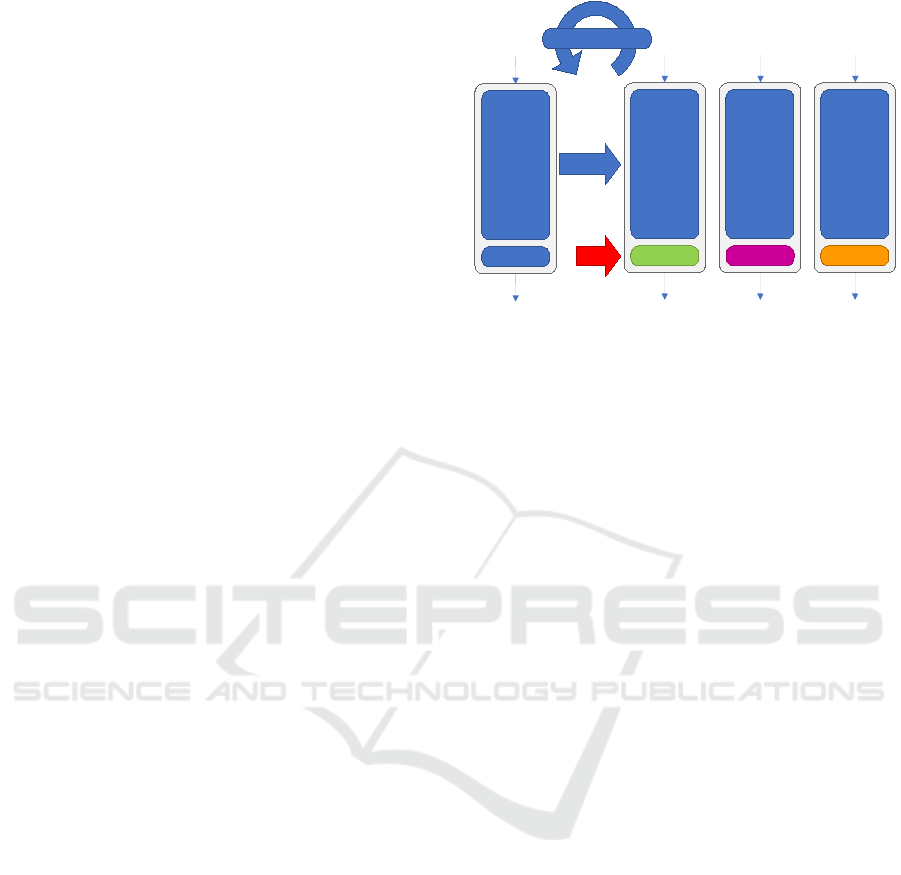
3.2.1 Train Strategies
The training of a classifier ensemble is conducted
in multiple steps. Initially, a base model is created
and trained on the training dataset, after which it is
saved. Subsequently, a new base model is created,
and the weights from the previously trained model are
loaded. Following the principles of transfer learning,
the weights are frozen, and only the head is newly
constructed and then trained again on the training
data. This process is repeated as many times as nec-
essary to form the desired number of heads for the
classifier ensemble, as illustrated in Figure 3.
Such a separate training approach offers several
advantages. It allows the use of different head archi-
tectures, such as varying the number of layers or in-
corporating dropout. Additionally, diverse data aug-
mentation strategies or different subsets of the dataset
can be applied during each head’s training, akin to the
bagging ensemble method described in Section 2.
3.2.2 Ensemble Methods
In the final step of the classifier ensemble, the differ-
ent heads must be combined, as shown in Figure 2.
Our proposed methods for combining these heads in-
clude averaging, voting, and the use of metamodels.
Averaging involves summing the individual outputs
of the heads and dividing the total by the number of
heads. In voting, a majority decision is made by se-
lecting the most frequent predicted values across the
heads.
Alternatively, metamodels can be used, where the
classifiers are combined using additional learnable
Backbone
Head
Head 1 Head m...
Training set
Backbone
frozen
Backbone
frozen
Backbone
frozen
load
new
Figure 3: Training Process of our classifier ensemble.
parameters. One approach involves concatenating the
outputs of all m heads and applying a fully connected
layer, where the input consists of the combined pre-
dictions from the heads, yielding m · C input features,
while the output remains the original C classes.
The architecture can be further extended with ad-
ditional hidden layers, nonlinearities, or dropout, as
long as the structure supports m · C input and C out-
put features. Another variant is to link the head out-
puts class-wise with a fully connected layer. In this
case, a separate fully connected layer is used for each
class, with each layer having m input features and a
single output, leading to a total of C fully connected
layers, one for each class.
In the studies conducted in Section 4.2, we per-
formed a thorough comparison of all methods. How-
ever, no single approach consistently outperformed
the others across different networks and datasets.
Nevertheless, all methods demonstrated a significant
improvement compared to the uncalibrated baseline.
4 EVALUATION
Our evaluation is divided into three sections. Section
4.1 first provides a detailed overview of the data and
training settings used for all our experiments. Next,
in section 4.2.1, we conduct an extensive study with
CIFAR-100 (Krizhevsky et al., 2009). Finally, in Sec-
tion 4.2.2, we use Tiny ImageNet (Le and Yang, 2015)
for further evaluations.
4.1 Datasets, Training, and Ensemble
Configuration
Datasets. To evaluate our novel classifier ensemble,
we utilize the CIFAR-100 (Krizhevsky et al., 2009)
dataset. CIFAR-100 consists of 50,000 training im-
Classifier Ensemble for Efficient Uncertainty Calibration of Deep Neural Networks for Image Classification
319

Table 1: Comparison of accuracy, ECE and MCE in percent of uncalibrated heads and their combination to the classifier
ensemble with ResNet (He et al., 2016) variants on CIFAR-100 (Krizhevsky et al., 2009).
Model
ResNet18 ResNet34 ResNet50 ResNet101
Acc. ECE MCE Acc. ECE MCE Acc. ECE MCE Acc. ECE MCE
Baseline
Head 1 75.08 4.41 27.47 76.74 5.60 15.66 77.21 8.22 25.01 78.06 8.76 21.06
Head 2 74.95 4.69 16.26 76.76 5.74 15.00 77.15 8.30 23.80 78.06 8.83 23.14
Head 3 75.07 4.65 27.25 76.86 5.56 27.76 77.45 8.06 23.73 78.12 8.68 22.40
Head 4 75.22 4.40 24.07 76.89 5.92 17.64 77.39 8.04 25.96 78.20 8.64 23.26
Head 5 75.25 4.46 14.11 76.71 5.75 15.20 77.06 8.43 25.51 78.05 8.76 23.11
Classifier
Ensemble (ours)
Avg. 75.06 4.43 10.66 76.83 5.75 19.12 77.28 7.75 25.13 78.07 8.43 20.17
Vot. 74.96 4.25 11.97 76.81 5.12 14.27 77.29 7.58 24.97 77.99 8.31 22.85
SL 74.39 2.59 8.35 76.45 3.48 11.37 77.17 3.64 9.62 77.30 2.81 8.61
DL 74.29 2.93 8.44 76.37 3.44 9.10 76.89 4.00 10.52 77.44 2.71 7.57
DLL 74.73 3.51 10.22 76.75 3.83 11.12 77.32 3.12 11.10 77.94 3.39 10.66
SLpC 74.99 4.11 11.71 76.73 4.01 7.73 77.11 3.10 9.35 78.22 3.70 9.12
ages and 10,000 test images with 100 classes. In addi-
tion to the experiments on the CIFAR-100 dataset, we
also conducted experiments on the Tiny ImageNet (Le
and Yang, 2015) dataset consisting of 100,000 train-
ing images and 5,000 test images of 200 classes.
Base Training. As outlined in Section 3, the first step
in training our classifier ensemble is the standard pre-
training of a base model (backbone + head), which
serves as the foundation for subsequent steps. For this
work, a Stochastic Gradient Descent (SGD) optimizer
with momentum of 0.9 and weight decay of 5e-04 is
used. During the 200 training epochs, the basic learn-
ing rate of 0.1 is gradually adjusted by a factor of 0.2
using a multi-stage scheduler. A batch size of 128 and
a basic data augmentation strategy, including random
cropping, padding, horizontal flipping and random ro-
tation is used.
Training Heads. The individual heads are created by
loading the base model. As described in Section 3,
the backbone weights are frozen and only the clas-
sifier (head) is reinitialized with new random seeds.
The new classifier is then trained using an SGD opti-
mizer with an initial learning rate of 0.1. The learning
rate for training the heads is adjusted using a Plateau-
Min-Scheduler, which monitors the validation loss. If
the loss does not improve within a specified number
of epochs, the learning rate is reduced by multiply-
ing it by a factor of 0.5. Additionally, early stopping
with a patience of 15 epochs is applied, terminating
the training if no further improvements are observed.
All heads used in this work consist of a single fully
connected layer. Each base model is trained with five
distinct heads, which are saved and later combined
into an ensemble. Since each head contains only a
few parameters, the training process is very fast.
Ensemble Configuration. For classifier ensemble
without a metamodel, two combination methods were
explored: mean averaging and majority voting. When
using a metamodel to combine the heads, additional
training is required. Four metamodels were imple-
mented and analyzed: Single-Layer (SL), Double-
Layer (DL), Double-Layer-Large (DLL), and Single-
Layer-per-Class (SLpC).
The SL metamodel combines the outputs of the
heads through a single fully connected layer. The DL
metamodel adds a second layer with ReLU activation
and dropout, where the first layer reduces the number
of neurons. In contrast, the DLL metamodel doubles
the number of neurons in the first layer compared to
the DL model. The SLpC metamodel takes a different
approach, using a dedicated fully connected layer for
each class, where the concatenated head outputs are
connected with class-specific layers.
As the metamodels introduce additional parame-
ters, they require training on the training dataset. This
training is performed over 20 epochs using an SGD
optimizer with an initial learning rate of 0.0002, along
with a Plateau-Min-Scheduler to adjust the learning
rate. After training, the metamodel with the lowest
validation loss is selected for deployment.
4.2 Results
Eight different base models were developed and
trained on the CIFAR-100 dataset, with five distinct
heads trained for each base model. The results for
various ResNet models (He et al., 2016) are dis-
played in Table 1, while more advanced models such
as DenseNets (Huang et al., 2017), ResNeXt (Xie
et al., 2017) and GoogLeNet (Szegedy et al., 2015)
are shown in Table 2. All heads were combined with
our classifier ensembles using different methods, in-
cluding mean averaging, majority voting and different
metamodels called Single-Layer (SL), Double-Layer
VISAPP 2025 - 20th International Conference on Computer Vision Theory and Applications
320

Table 2: Comparison of accuracy, ECE and MCE in percent of uncalibrated heads and their combination to the classifier
ensemble with ResNeXt (Xie et al., 2017), DenseNet (Huang et al., 2017) and GoogLeNet (Szegedy et al., 2015) on CIFAR-
100 (Krizhevsky et al., 2009).
Model
ResNeXt50 DenseNet121 DenseNet169 GoogLeNet
Acc. ECE MCE Acc. ECE MCE Acc. ECE MCE Acc. ECE MCE
Baseline
Head 1 77.15 6.05 15.06 77.55 4.74 10.20 78.43 4.00 10.28 75.66 6.93 16.65
Head 2 77.06 5.99 12.28 77.45 4.75 12.02 78.56 3.92 9.30 75.84 7.02 19.36
Head 3 76.86 6.14 13.56 77.55 4.97 13.04 78.57 4.08 9.64 75.74 6.96 18.68
Head 4 76.91 6.34 16.08 77.43 4.70 10.49 78.42 4.05 9.02 75.71 7.04 18.88
Head 5 77.27 5.96 15.09 77.49 4.49 11.75 78.51 4.04 8.60 75.66 7.07 19.15
Classifier
Ensemble (ours)
Avg. 77.13 5.63 13.26 77.56 4.27 9.77 78.44 3.68 8.85 75.74 6.72 17.35
Vot. 76.99 5.52 13.55 77.52 4.29 10.41 78.53 3.61 8.21 75.77 6.37 15.74
SL 76.45 2.66 7.53 77.27 2.95 11.51 78.24 2.46 8.05 75.09 3.55 7.94
DL 76.27 2.07 5.97 77.18 2.69 19.08 77.66 2.23 8.88 75.36 4.44 8.68
DLL 76.57 3.24 9.57 77.51 2.79 11.58 78.09 2.19 8.86 75.43 4.84 10.36
SLpC 77.22 2.80 8.99 77.39 2.95 7.86 78.56 3.09 10.88 75.73 4.91 10.32
(DL), Double-Layer Large (DLL) and Single-Layer
per Class (SLpC). The tables summarize the results
for architectures, highlighting accuracy (Acc.), Ex-
pected Calibration Error (ECE), and Maximum Cal-
ibration Error (MCE). Individual heads are presented
as baseline, where each head paired with the back-
bone represents a different variation due to the unique
random seed applied. The tables present the results
for mean averaging and majority voting, followed by
the outcomes of the trained metamodels.
4.2.1 Results for CIFAR-100
The results across different ResNet variants on
CIFAR-100 (see Table 1) reveal a consistent trend.
For individual heads, the accuracy remains fairly con-
sistent across all ResNet models, with ResNet101
achieving the highest accuracy (78.22%). How-
ever, this also corresponds with higher ECE and
MCE values, indicating issues with model calibration.
Mean averaging as an ensemble method yields slight
improvements in accuracy and moderate reductions
in ECE, particularly in ResNet50 and ResNet101,
though the calibration improvements are not substan-
tial. Majority voting offers better calibration than
mean averaging, resulting in lower ECE and MCE,
but accuracy is marginally lower compared to mean
averaging.
The metamodels, particularly the SL and DL ap-
proaches, show the most significant reductions in
ECE and MCE across all ResNet variants, especially
for ResNet101. Although these methods slightly de-
crease accuracy, the calibration improvement is sub-
stantial. The DLL and SLpC models also exhibit
strong calibration performance, with SLpC perform-
ing notably well in terms of ECE for ResNet50.
Table 3: Comparison of accuracy, ECE and MCE in percent
of classic model ensemble with ResNet18 (He et al., 2016)
on CIFAR-100 (Krizhevsky et al., 2009).
Model
ResNet18
Acc. ECE MCE Params
Model 1 74.89 5.96 27.61 11.22 M
Model 2 75.03 6.26 17.23 11.22 M
Model 3 74.20 9.72 22.02 11.22 M
Model 4 73.08 11.30 25.82 11.22 M
Model 5 71.66 7.98 18.26 11.22 M
Ensemble 75.85 6.91 18.32 56.10 M
In line with the findings in Table 1 for ResNet vari-
ants, the more advanced models presented in Table 2
display a comparable pattern. While individual heads
achieve competitive accuracy, they consistently ex-
hibit higher calibration errors, with GoogLeNet show-
ing particularly elevated ECE and MCE values.
Mean averaging and majority voting marginally
reduce calibration errors across all models, particu-
larly in DenseNet and ResNeXt. However, these re-
ductions are not as significant as those seen with the
use of metamodels. The trained metamodels, partic-
ularly the DL and SL approaches, yield substantial
improvements in calibration metrics. The DL meta-
model delivers the lowest ECE and MCE values for
ResNeXt and DenseNet, with notable performance in
reducing calibration errors while maintaining accu-
racy. The SLpC model also demonstrates good cal-
ibration, especially for DenseNet169, which achieves
a balance between low ECE and high accuracy.
Compared to the previous table for ResNet mod-
els, these results further highlight the effectiveness of
classifier ensembles with metamodels in reducing cal-
ibration errors, with DL consistently performing well
Classifier Ensemble for Efficient Uncertainty Calibration of Deep Neural Networks for Image Classification
321

across architectures. However, the trade-off between
accuracy and calibration remains present, as seen with
the slight dip in accuracy in some metamodel ap-
proaches. Overall, classifier ensembles incorporating
metamodels continue to significantly enhance model
calibration across various architectures, building on
the trends observed with the ResNet variants.
As reference, a traditional horizontal model en-
semble using ResNet18 was also evaluated. The re-
sults are shown in Table 3. This approach aggregates
models from different checkpoints during training and
combines their outputs using mean averaging. When
comparing the ResNet18 results from Table 3 with
those in Table 1, some distinct trends can be observed.
The accuracy of the classical model ensemble in
Table 3 reaches 75.85%, which is slightly higher than
the individual heads, where the highest accuracy is
75.25%. However, the calibration errors, particularly
the ECE and MCE, remain relatively high in the clas-
sical ensemble, with 6.91% and 18.32%, respectively.
In contrast, our classifier ensembles using metamod-
els in Table 1 consistently achieve much lower cali-
bration errors, with the SL and DL approaches reduc-
ing the ECE to 2.59% and 2.93%, respectively, while
also minimizing the MCE.
Another notable difference is the parameter count.
The classical ensemble significantly increases the
number of parameters to 56.1 M, whereas the clas-
sifier ensembles with metamodels only introduce mi-
nor increases in parameter count (approximately 3%).
Thus, while the classical ensemble offers slightly im-
proved accuracy, it does so at the cost of significantly
higher calibration errors and a substantial increase in
model size compared to the classifier ensemble meth-
ods.
4.2.2 Results for Tiny ImageNet
Table 4 presents the results of ResNet18 trained on the
Tiny ImageNet dataset, comparing individual heads
and various classifier ensemble methods in terms of
accuracy (Acc.), Expected Calibration Error (ECE)
and Maximum Calibration Error (MCE).
The individual heads achieve accuracy scores
around 63.3%, with ECE values between 5.84% and
6.43%, and MCE values ranging from 15.33% to
18.06%. The classifier ensemble methods reduce cal-
ibration errors, with the DLL approach notably low-
ering the ECE to 3.13% and MCE to 6.62%, signif-
icantly outperforming the other methods in terms of
calibration. However, the accuracy of the ensemble
methods slightly decreases compared to the individ-
ual heads.
Table 4: Comparison of accuracy, ECE and MCE in percent
of uncalibrated heads and their combination to the classi-
fier ensemble with ResNet18 (He et al., 2016) on Tiny Ima-
geNet (Le and Yang, 2015).
Model
ResNet18
Acc. ECE MCE
Baseline
Head 1 63.41 6.02 16.56
Head 2 63.11 5.91 15.33
Head 3 63.23 6.43 18.06
Head 4 63.39 6.05 15.89
Head 5 63.34 5.84 17.09
Classifier
Ensemble (ours)
Avg. 63.32 5.86 16.43
Vot. 63.32 5.67 14.65
SL 62.69 5.00 11.35
DL 62.05 5.09 13.19
DLL 62.58 3.13 6.62
SLpC 63.26 4.92 8.93
5 CONCLUSIONS
In this study, we explored various ensemble tech-
niques using multiple deep learning architectures on
the CIFAR-100 and Tiny ImageNet datasets. Our fo-
cus was on evaluating the accuracy and calibration
performance of our novel classifier ensembles, partic-
ularly in reducing Expected Calibration Error (ECE)
and Maximum Calibration Error (MCE).
The results show that while individual heads
achieve reasonable accuracy, they often exhibit high
calibration errors, particularly on larger models. Sim-
ple ensemble techniques such as mean averaging and
majority voting provide modest improvements in cal-
ibration but fail to significantly lower the ECE and
MCE. In contrast, metamodel-based ensemble meth-
ods consistently outperform these basic techniques
in terms of calibration, with our Double-Layer and
Double-Layer Large methods beeing particularly ef-
fective in reducing both ECE and MCE, albeit with
slight reductions in accuracy.
Compared to traditional model ensembles, classi-
fier ensembles with metamodels demonstrated similar
improvements in calibration with far fewer parame-
ters, offering a more efficient approach to improving
model reliability. These findings suggest that integrat-
ing metamodels into classifier ensembles can provide
a robust solution for enhancing the calibration of deep
learning models, making them more reliable in real-
world applications.
Future work could explore the scalability of these
methods to even larger datasets and architectures, as
well as their potential in more complex tasks like ob-
ject detection requiring highly calibrated predictions.
VISAPP 2025 - 20th International Conference on Computer Vision Theory and Applications
322

ACKNOWLEDGEMENTS
This research was partly funded by Albert and An-
neliese Konanz Foundation, the German Research
Foundation under grant INST874/9-1 and the Federal
Ministry of Education and Research Germany in the
project M
2
Aind-DeepLearning (13FH8I08IA).
REFERENCES
Br
¨
ocker, J. (2009). Reliability, sufficiency, and the decom-
position of proper scores. Quarterly Journal of the
Royal Meteorological Society.
Ebert, N., Mangat, P., and Wasenm
¨
uller, O. (2022). Multi-
task network for joint object detection, semantic seg-
mentation and human pose estimation in vehicle occu-
pancy monitoring. In Intelligent Vehicles Symposium
(IV).
Ebert, N., Stricker, D., and Wasenm
¨
uller, O. (2023).
Transformer-based detection of microorganisms on
high-resolution petri dish images. In International
Conference on Computer Vision Workshops (ICCVW).
Gal, Y. and Ghahramani, Z. (2016). Dropout as a bayesian
approximation: Representing model uncertainty in
deep learning. In International Conference on Ma-
chine Learning (ICML).
Goodfellow, I. (2016). Deep learning.
Guo, C., Pleiss, G., Sun, Y., and Weinberger, K. Q. (2017).
On calibration of modern neural networks. In Inter-
national Conference on Machine Learning (ICML).
He, K., Zhang, X., Ren, S., and Sun, J. (2016). Deep resid-
ual learning for image recognition. In Conference on
Computer Vision and Pattern Recognition (CVPR).
Huang, G., Liu, Z., Van Der Maaten, L., and Weinberger,
K. Q. (2017). Densely connected convolutional net-
works. In Conference on Computer Vision and Pattern
Recognition (CVPR).
Jiang, H., Kim, B., Guan, M., and Gupta, M. (2018). To
trust or not to trust a classifier. Advances in Neural
Information Processing Systems (NeurIPS).
Kendall, A. and Gal, Y. (2017). What uncertainties do we
need in bayesian deep learning for computer vision?
Advances in Neural Information Processing Systems
(NeurIPS).
Krizhevsky, A., Hinton, G., et al. (2009). Learning multiple
layers of features from tiny images. Technical report.
Kumar, A., Sarawagi, S., and Jain, U. (2018). Trainable
calibration measures for neural networks from kernel
mean embeddings. In International Conference on
Machine Learning (ICML).
Lakshminarayanan, B., Pritzel, A., and Blundell, C. (2017).
Simple and scalable predictive uncertainty estimation
using deep ensembles. Advances in Neural Informa-
tion Processing Systems (NeurIPS).
Le, Y. and Yang, X. (2015). Tiny imagenet visual recogni-
tion challenge. CS 231N.
Naeini, M. P., Cooper, G., and Hauskrecht, M. (2015).
Obtaining well calibrated probabilities using bayesian
binning. In AAAI Conference on Artificial Intelli-
gence.
Niculescu-Mizil, A. and Caruana, R. (2005). Predicting
good probabilities with supervised learning. In Inter-
national Conference on Machine Learning (ICML).
Oehri, S., Ebert, N., Abdullah, A., Stricker, D., and
Wasenm
¨
uller, O. (2024). Genformer – generated im-
ages are all you need to improve robustness of trans-
formers on small datasets. In International Confer-
ence on Pattern Recognition (ICPR).
Platt, J. et al. (1999). Probabilistic outputs for support vec-
tor machines and comparisons to regularized likeli-
hood methods. Advances in Large Margin Classifiers.
Raschka, S., Liu, Y. H., and Mirjalili, V. (2022). Ma-
chine Learning with PyTorch and Scikit-Learn: De-
velop machine learning and deep learning models
with Python. Packt Publishing Ltd.
Reichardt, L., Ebert, N., and Wasenm
¨
uller, O. (2023).
360deg from a single camera: A few-shot approach
for lidar segmentation. In International Conference
on Computer Vision Workshops (ICCVW).
Szegedy, C., Liu, W., Jia, Y., Sermanet, P., Reed, S.,
Anguelov, D., Erhan, D., Vanhoucke, V., and Rabi-
novich, A. (2015). Going deeper with convolutions. In
Conference on Computer Vision and Pattern Recogni-
tion (CVPR).
Tomani, C., Cremers, D., and Buettner, F. (2022). Param-
eterized temperature scaling for boosting the expres-
sive power in post-hoc uncertainty calibration. In Eu-
ropean Conference on Computer Vision.
Wenzel, F., Snoek, J., Tran, D., and Jenatton, R. (2020).
Hyperparameter ensembles for robustness and uncer-
tainty quantification. Advances in Neural Information
Processing Systems (NeurIPS).
Xie, S., Girshick, R., Doll
´
ar, P., Tu, Z., and He, K. (2017).
Aggregated residual transformations for deep neural
networks. In Conference on Computer Vision and Pat-
tern Recognition (CVPR).
Zadrozny, B. and Elkan, C. (2001). Learning and making
decisions when costs and probabilities are both un-
known. In International Conference on Knowledge
Discovery and Data Mining.
Zadrozny, B. and Elkan, C. (2002). Transforming classifier
scores into accurate multiclass probability estimates.
In International Conference on Knowledge Discovery
and Data Mining.
Zhang, J., Kailkhura, B., and Han, T. Y.-J. (2020). Mix-n-
match: Ensemble and compositional methods for un-
certainty calibration in deep learning. In International
Conference on Machine Learning (ICML).
Classifier Ensemble for Efficient Uncertainty Calibration of Deep Neural Networks for Image Classification
323