Multiple Crack Detection in Beam-Like Structures Using a Novel

Particle Swarm Optimization Approach

Flaviu-Catalin Florea

4 a

, Horea Grebla

1 b

, Gilbert-Rainer Gillich

2 c

Bogdan Nicus

or Bindea

5 d

and Catalin V. Rusu

1,3 e

Department of Computer-Science, Babes-Bolyai University, Romania

Department of Engineering Science, Babes-Bolyai University, Romania

Department of Computer Science, Institute of German Studies, Babes-Bolyai University, Romania

Department of Computer Science, Aarhus University, Denmark

Department of Computer Science, Technical University of Cluj-Napoca, Romania

Keywords:

Damage Detection, Natural Frequencies, Cost Function, Particle Swarm Optimization.

Abstract:

This paper presents a method for assessing two cracks in simply supported beams by identifying their locations

and severities (depths). Our method is based on applying the Particle Swarm Optimization (PSO) algorithm

with the measured natural frequencies for several bending vibration modes of an intact and cracked beam. We

are using calculated relative frequency shifts (RFS) for eight vibration modes for all possible damage cases

using a mathematical relation deduced in previous researches. We detect changes, calculate the RFSs and

then subtract, separately for all modes, the measured RFSs from all calculated RFSs. Considering previously

demonstrated applications of PSO for one crack detection, we propose strategies to enable PSO to determine

locations in scenarios involving two cracks. Our method is successful in accurately identifying two damage

locations and severities.

1 INTRODUCTION

Fault detection in beam-like structures is an important

research ﬁeld as it has real-life implications, from sav-

ing time, money and even lives, if cracks are detected

in early stages. There are several studies that use non

invasive methods to identify the location and depth of

one crack in beam like structures. There are however

only a few such studies that deal with multiple cracks

at the same time. Most related work involving Evo-

lutionary Algorithms focuses on Genetic Algorithms

(GA), but in this study our focus is on Particle Swarm

Optimization (PSO). To our knowledge, no prior work

uses the Equivalent Healthy Beam (EHB) model with

Evolutionary Algorithms for damage prediction.

Mohan, Maiti and Maity evaluated PSO and GA

in multiple crack detection (Mohan et al., 2013). PSO

outperformed GA in accuracy and robustness, consis-

tently providing more reliable predictions. They used

the Frequency Response Function (FRF) model on a

https://orcid.org/0009-0009-2479-6588

https://orcid.org/0000-0002-8529-5797

https://orcid.org/0000-0003-4962-2567

https://orcid.org/0009-0000-7045-2043

https://orcid.org/0000-0002-2056-8440

simple cantilever beam, demonstrating that combin-

ing FRF with PSO enhances accuracy. Khatir et al.

(Khatir et al., 2017) also compared GA and PSO for

detecting cracks in composite beams. PSO proved su-

perior in accuracy, efﬁciency, and robustness, espe-

cially with noise in the modal data, guiding the objec-

tive function using the Modal Assurance Criterion.

Greco et al. (Greco et al., 2018) proposed a static

method using GA and a closed-form solution based

on a rotational spring model for multiple crack detec-

tion. This method, implemented in the NetLogo en-

vironment, showed effective crack identiﬁcation un-

der various conditions. Khai and Mehrjoo (Khaji and

Mehrjoo, 2014) introduced a new beam element capa-

ble of including multiple transverse edge cracks. Us-

ing GA, they solved an inverse problem to determine

crack speciﬁcs, validating their method against 2D ﬁ-

nite element analyses and experimental data. Zheng,

Liang, Wang and Fan (Zheng et al., 2014) used a Hi-

erarchical Genetic Algorithm (HGA) with the same

model as the one used in (Khaji and Mehrjoo, 2014),

proving HGA’s superiority over simple GA in reduc-

ing ﬁnite element computations and avoiding prema-

ture convergence. Sahu, Kumar, and Parhi developed

a hybrid method (CSAGA) combining GA with the

334

Florea, F.-C., Grebla, H., Gillich, G.-R., Bindea, B. N. and Rusu, C. V.

Multiple Crack Detection in Beam-Like Structures Using a Novel Particle Swarm Optimization Approach.

DOI: 10.5220/0013131400003890

Paper published under CC license (CC BY-NC-ND 4.0)

In Proceedings of the 17th International Conference on Agents and Artiﬁcial Intelligence (ICAART 2025) - Volume 3, pages 334-342

ISBN: 978-989-758-737-5; ISSN: 2184-433X

clonal selection algorithm (Sahu et al., 2018). This

method improved accuracy in locating cracks and as-

sessing their severity by examining changes in natural

frequencies. Moradi and Kargozarfard (Moradi and

Kargozarfard, 2013) introduced the Bees Algorithm

for multiple crack detection, using changes in eigen-

frequencies and strain energy parameters to optimize

a damage index vector. This method effectively iden-

tiﬁed the number and locations of cracks.

Machine learning approaches, primarily using Ar-

tiﬁcial Neural Networks (ANN), are less common

in crack detection. Maurya, Mishra and Panigrahi

demonstrated ANN’s effectiveness in structural anal-

ysis, using the ﬁrst three relative natural frequen-

cies to predict crack locations and depths accurately

(Maurya et al., 2018). Pop, Tuﬁsi, and Gillich (Pop

et al., 2022) optimized an ANN through feedfor-

ward backpropagation to pinpoint crack positions in

a 1000mm cantilever steel beam with high precision.

Their model utilized the ﬁrst ﬁve natural frequencies,

highlighting the impact of crack proximity on modal

response.

In multiple crack detection for beam-like struc-

tures, GAs and the rotational spring model are pre-

dominant. However, each study achieves different

error percentages based on varying beam properties,

making direct comparisons difﬁcult. Most studies re-

port errors close to 2%, 1%, or even 0%.

Nevertheless, we found no study up to date to

tackle the problem from the point of view of the

Equivalent Healthy Beam model and Particle Swarm

Optimization. Hence, we propose a new approach for

multiple damage detection.

2 THEORETICAL BACKGROUND

2.1 Particle Swarm Optimization

Particle Swarm Optimization (PSO) is a method

within evolutionary computation in artiﬁcial intelli-

gence (AI), inspired by natural behaviors such as bird

ﬂocking and ﬁsh schooling. Imagine a ﬂock of birds:

when one bird ﬁnds a good spot for food, others fol-

low, adjusting their paths. Similarly, in PSO, each

”particle” (representing a potential solution) moves

through the solution space, learning from its own ex-

periences and those of others. Each particle keeps

track of its best position and is inﬂuenced by the best

position found by the swarm.

PSO success hinges on balancing exploration

(scouting new areas) and exploitation (reﬁning known

good areas). This balance is managed through key

settings:

• Inertia Weight (w): Helps particles move. A

higher weight in the early stages encourages broad

exploration, while a reduced weight later on helps

ﬁne-tune solutions.

• Cognitive Coefﬁcient (c1): Inﬂuences a particle

based on its past success, encouraging it to revisit

or stay near promising solutions.

• Social Coefﬁcient (c2): Inﬂuences a particle

based on the swarm’s best-found solution, pro-

moting a collective approach.

The velocity and position of each particle are up-

dated using:

k+1

= w ·v

+ c1 ·r1

·(pbest

−x

) + c2 ·r2) ·(gbest −x

) (1)

= x

+ v

k+1

(2)

where v

and v

k+1

are the current and next veloc-

ities of particle i, w is the inertia parameter, c1 is the

cognitive parameter, c2 is the social parameter, pbest

is the best position of particle i, gbest is the best posi-

tion of the swarm, x

is the current position of particle

i, and r1 and r2 are random numbers between 0 and

Topology, which dictates how particles commu-

nicate, is crucial in Particle Swarm Optimization.

Within a global topology, every particle communi-

cates with all others, quickly sharing the best solu-

tions. In contrast, a local topology restricts commu-

nication to nearby particles, encouraging more inde-

pendent exploration. This choice affects how swiftly

the swarm converges and how well it ﬁnds optimal

solutions.

We will go into more depth about the steps we

took to get our PSO model to correctly anticipate two

defects in a cantilever beam in the upcoming chapters.

The techniques and experiments, ranging from hyper-

parameter tweaking to several unique approaches, are

covered in the next chapters.

2.2 Relative Frequency Shift for One

Crack Scenario

A crack in a beam decreases the rigidity of a speciﬁc

area, affecting its vibration. This is seen as changes in

eigenfrequencies, which are the natural vibration fre-

quencies of the structure. For a thought experiment,

imagine a cantilever beam, ﬁxed at one end and free at

the other. If one were to push it down on the free end

and then release it, the beam will vibrate at a speciﬁc

frequency. If there is a crack at a point c with depth

Multiple Crack Detection in Beam-Like Structures Using a Novel Particle Swarm Optimization Approach

335

d, the beam will be weaker at that point, causing it to

bend more under the same pressure.

To model this, we use the Equivalent Healthy

Beam (EHB) model (Gillich et al., 2019). This model

suggests that a beam with a crack behaves like a thin-

ner, uniformly healthy beam with the same deﬂection

at the free end. According to Castigliano’s theorem,

both beams store the same energy and oscillate at the

same frequency.

The relationship between the deﬂection δ at the

free end and the eigenfrequency f

is:

2π

8δ

(3)

where λ

is the eigenvalue for each i vibration

mode and g is the gravitational constant. The deﬂec-

tion δ for the healthy beam is:

δ =

pgAL

8EI

(4)

where L is the length of the beam, A is the cross-

sectional area (A = width×height), p is the mass den-

sity, E is the Young’s modulus, and I is the moment

of inertia. The constant 8 comes from the boundary

conditions of the beam (Gillich et al., 2021).

Cracks deepen at point c to d, making the free

end bend more (δ(c,d)). The healthy beam needs less

area (A(c,d)) and less bending resistance (I(c,d)) to

match. Both vibrate the same because they store the

same energy, and you calculate the damaged beam’s

frequency like this:

(c,d) =

2π

8δ(c,d)

(5)

This leads to:

(c,d) = f

δ(c,d)

(6)

A crack at c = 0, where the curvature is maxi-

mum, will cause the greatest increase in deﬂection

and the largest decrease in frequency. In the litera-

ture, it’s called the Equivalent Healthy Beam (EHB).

It’s the least stiff among healthy beams used to model

a crack of a certain depth. We assign a damage sever-

ity coefﬁcient, γ, to the crack, calculated as shown in

(Praisach et al., 2013).

γ(0,d) =

δ(0,d) −

√

δ(0,d)

(7)

As shown in Figure 1, a beam with a crack at lo-

cation c has higher deﬂection than a healthy beam but

the same deﬂection as an EHB with the crack at c = 0.

Figure 1: The 2 models of a beam; one with a crack at loca-

tion c and one with the crack at the ﬁxed end.

The frequency drop ∆ f

for a crack at c = 0 is:

∆ f

(0,d) = f

− f

(0,d) = f

1 −

δ(0,d)

= f

δ(0,d) −

√

δ(0,d)

= f

γ(0,d)

(8)

For a general crack position c:

∆ f

(c,d) = f

− f i(c, d) = f

δ(c,d) −

√

δ(c,d)

(9)

The damage severity γ can be related to the

normalized modal curvature



”

(c)



(Gillich and

Praisach, 2014):

γ(c,d) =

δ(c,d) −

√

δ(c,d)

δ(0,d) −

√

δ(0,d)



”

(c)



= γ(0,d)



”

(c)



(10)

where



”

(c)



is the normalized modal curvature,

indicating the local curvature’s effect due to bending.

For cantilever beams, the normalized curvature is:

”

(x) = 0.5

{

cos(λ

x) + cosh(λ

−

cos(λ

) + cosh(λ

)

sin(λ

) + sinh(λ

)

(sin(λ

x) + sinh(λ

x))



(11)

The frequency drop for a crack at c is:

∆ f

(c,d) = f

·γ(0,d) ·



”

(c)



(12)

The Relative Frequency Shift (RFS) for a can-

tilever beam with one crack is:

∆ f

(c,d) = γ(0,d)·



”

(c)



(13)

This allows quick calculation of RFS for any crack

depth and location, crucial for our PSO model.

ICAART 2025 - 17th International Conference on Agents and Artiﬁcial Intelligence

336

2.3 Relative Frequency Shift for

Multiple Cracks Scenario

When multiple cracks are present, each crack inde-

pendently alters the stiffness of the beam and affects

modal parameters, such as natural frequencies, mode

shapes and damping factors. If the cracks are sufﬁ-

ciently far apart (more than 5mm), the superposition

principle applies, allowing the effects to be consid-

ered independently (Gillich et al., 2021).

The total RFS for two cracks is:

∆ f

(c1,d1,c2,d2) = ∆ f

(c1,d1) + ∆ f

(c2,d2) (14)

Experiments show that for cracks at least 5mm

apart, the EHB model applies with less than 0.005%

error (Gillich et al., 2021).

In our study, we use these relations to calculate

RFSs for any crack combination. This allows us to

train our PSO model on various crack scenarios, solv-

ing the optimization problem of identifying damage

properties from RFS data.

3 APPROACH AND

METHODOLOGY

For our simulations we will consider a cantilever

beam of 1000mm in length and a depth of 20mm.

We will be using a GeneralOptimizer PSO from

the Pyswarms library (PYS, ) as our PSO model. The

following is the form of the objective function that the

model must optimize:

f (solution) = −



∑

i=1

(RFS

(solution) −InputRFS

)



−5

(15)

where RFS

is the function from equation 14, i de-

notes the frequency modes, the solution denotes two

places and two depths for the cracks, and InputRFS

denotes the relative frequencies shifts received as in-

put for the fractured beam.

Going forward, whenever we discuss the charac-

teristics of a fractured beam (or target) using a 4-value

array such as [0.12, 0.65, 0.34, 1.34], the ﬁrst two val-

ues, 0.12 and 0.65, denote the locations of the cracks

on a scale ranging from 0 to 1, while the ﬁnal two val-

ues, 0.34 and 1.34, represent the depths of the cracks

on a scale ranging from 0 to 2. For locations, the

boundaries of the space search are therefore [0 - 1]

and for depths, [0 - 2]. The RFS equation will be used

to construct the InputRFS

when we test our model by

creating random targets using the previously outlined

structure.

The following formula is used to calculate the er-

ror:

err(predicted) =

|predicted −real|

length of interval

∗100 (16)

The length of the interval is 1 −0 = 1 in the case

of location and 2 −0 = 2 in the case of depth.

3.1 Hyper-Parameters Tuning

We employed an exhaustive search (GridSearch) to

optimize the parameters c1, c2, and w. Initially, we

used 100 particles and 200 iterations, exploring the

range [0.0 - 1.0] for each parameter with a target of

[0.2, 0.3, 0.2, 0.1] and a Star topology. The opti-

mal parameters found were c1 = 0.4, c2 = 0.5, and

w = 0.1, but predictions with these settings were in-

consistent, with errors up to 80

To address this, we ran GridSearch on 48 random

targets, saving the parameters and costs after each run,

and computed weighted averages: c1 = 0.4, c2 = 0.6,

and w = 0.2. Despite the close similarity to the initial

results, the error remained unsatisfactory.

We manually tested a broader range of values, dis-

covering that higher c1 values improved performance

due to the function’s numerous local minima. Even-

tually, we identiﬁed c1 = 3, c2 = 0.25, and w = 0.5

as promising settings, occasionally achieving errors

close to 1%.

To validate these ﬁndings, a comprehensive Grid-

Search with c1 and c2 in [0.2 - 5] and w in [0.1

- 1.1] was conducted, targeting [0.05878, 0.08467,

0.49865, 0.25434]. The results, c1 = 4.2, c2 = 0.6,

and w = 1.0, conﬁrmed the need for higher c1. How-

ever, due to concerns about local minima, we retained

c1 = 3, c2 = 0.25, and w = 0.5. Despite these adjust-

ments, error rates varied from 0.5% to 36%.

Further experimentation revealed the Ring topol-

ogy to be more effective than the Star topology. The

Ring topology limits communication to a ﬁnite num-

ber of neighbours, enhancing exploration and reduc-

ing the risk of convergence to local minima. We found

that 50 neighbors per particle yielded the best results,

regardless of total particle count (100, 200, or 700).

Finally, increasing the number of iterations from

200 to 1000 and the total number of particles from

100 to 700 was necessary for proper convergence.

However, we later found that increasing the number

of particles to 700 was not the most effective strategy,

as will be discussed in the subsequent sections.

We conducted a comprehensive set of tests to

identify the subintervals where the model performs

well and where it encounters difﬁculties. The loca-

tion interval was divided into four subintervals: [0.0 -

0.1], [0.1 - 0.8], [0.8 - 0.9], and [0.9 - 1.0], while the

Multiple Crack Detection in Beam-Like Structures Using a Novel Particle Swarm Optimization Approach

337

depth interval was divided into: [0.0 - 0.1], [0.1 - 0.5],

[0.5 - 1.7], and [1.7 - 2.0]. We created 256 test cases

using these location and depth values.

The error for each test case was calculated by av-

eraging four errors (two for locations and two for

depths). The model exhibited signiﬁcant challenges

when the depth was near 0 or close to 2, which,

despite being practical for monitoring beam failure,

highlighted its limitations. The model performed bet-

ter for depths between 0.1 and 1.7, though inconsis-

tencies persisted.

Notably, the model struggled with locations near

the clamped end or the free end, particularly within

the intervals [0.0 - 0.1] and [0.9 - 1.0]. This indicates

speciﬁc areas where the model’s accuracy needs im-

provement.

3.2 Our Approach

Observations of the model’s performance indicated

that results varied signiﬁcantly for the same target,

with error rates ranging from less than 1% to over

10%. To address this inconsistency, we implemented

a strategy of running the model multiple times and

aggregating the results.

First, we determined that the model performed

similarly with 100 particles compared to 700 particles

if the number of iterations was increased. Thus, we

increased the iterations from 1000 to 3000 and ran the

model three and ﬁve times per target. This approach

improved overall performance but required subjective

interpretation to identify the best results from multi-

ple runs, as shown in Table 1.

Table 1: Multiple runs per target results.

# runs Error Location error Depth error

3 5.7517% 4.1953% 5.9317%

5 3.8481% 2.2716% 3.1317%

For instance, we could obtain the optimal number

for the ﬁrst location from the ﬁrst run of the model,

and the optimal number for the second location from

the third run, if we ran the model three times for a

target.

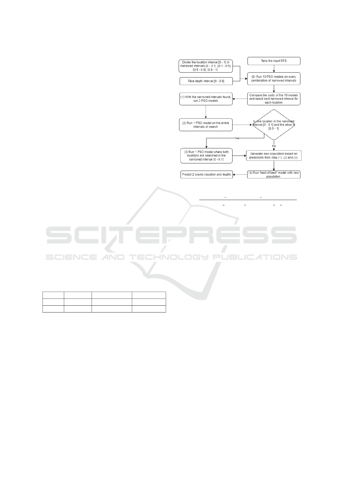
To address this shortcoming we developed a novel

”Best-of-Best” approach that involves merging out-

comes from various iterations and honing a swarm

population in order to create a new PSO model. Fig-

ure 2 shows our approach.

Our reﬁned PSO model thus creates a new swarm

population based on the best results from multiple

runs. For each result, we generated additional par-

ticles by slightly adjusting the predicted locations and

depths using a calculated step value, as in formula:

Figure 2: Flowchart of proposed algorithm.

step =

upper bound −lower bound + 3

additional particles needed//nr of results

(17)

where // is the ﬂoor division and the upper

ound

and lower

ound are the intervals of search. For ex-

ample, if we wanted to calculate the step for location,

given 10 results and a new population of 200, the step

would equal (1 −0 + 3)/(190//10) = 4/19 ≈ 0.21.

With this step, the new particles would be created by

adding to each predicted location a random number

from the interval (−step,step).

Our updated PSO model required appropriate

hyper-parameters, which we determined through

GridSearch and manual testing. We found that c1 = 3,

c2 = 0.2, and w = 0.4 worked best, with a Ring topol-

ogy and 40 neighbours. We also increased the number

of particles from 100 to 200.

Testing this new model, we ran it 5 and 10 times

for the same target, collected the results, and ran a ﬁ-

nal ”Best-of-Best” PSO model. Although the overall

performance error was not signiﬁcantly higher than

before, the location detection improved considerably,

achieving a low error of 0.71%, while depth detection

was less accurate at 4.79% in the 10 runs scenario (Ta-

ble 2, row 1 and 2).

The ”Best-of-Best” model not only selected the

best results from previous runs but also occasionally

identiﬁed better predictions by centring the new pop-

ulation around the prior best results.

ICAART 2025 - 17th International Conference on Agents and Artiﬁcial Intelligence

338

Table 2: Performance overview.

Nr. Runs on

entire

intervals

Runs

with

narrowed

intervals

Runs on

low locs

interval

Depth

narrowed

intervals

Y/N

Loc

bounds

Depth

bounds

Avg

err

Avg

loc

err

Avg

depth

err

1 5 - - - [0 - 1] [0 - 2] 5.96 2.93 8.99

2 10 - - - [0 - 1] [0 - 2] 2.75 0.71 4.79

3 2 5 1 or 3 Y [0 - 1] [0 - 2] 3.73 2.44 5.01

4 0 5 1 or 3 N [0 - 1] [0 - 2] 4.83 3.77 5.89

5 2 5 1 or 3 N [0 - 1] [0 - 2] 3.38 0.66 6.10

6 2 5 1 or 3 N [0 - 1] [0 - 1] 1.30 1.35 1.26

7 5 - - - [0 - 1] [0 - 1] 1.86 1.72 1.99

8 2 5 1 or 3 N [0 - 0.99] [0 - 1] 0.76 0.72 0.81

9 1 3 1 N [0 - 1] [0 - 0.3] 1.27 0.80 1.75

10 1 3 1 N [0 - 1] [0 - 0.6] 1.06 0.89 1.23

3.2.1 Improving the Performance Using

Narrowed Intervals of Search

One can however notice that the model’s error mar-

gin was minimal when it successfully identiﬁed the

target, but signiﬁcantly escalated (up to 30%) when

it failed. This led us to conclude that narrowing the

search intervals would improve precision. We divided

the location range [0 - 1] into four smaller intervals:

[0 - 0.1], [0.1 - 0.5], [0.5 - 0.9], and [0.9 - 1]. PSO

models were executed within these intervals, result-

ing in ten runs to cover all combinations. A similar

approach was applied to the depth range [0 - 2], di-

viding it into: [0.0 - 0.2], [0.2 - 1], [1 - 1.8], and [1.8

- 2].

Next, we ran 5 PSO models to search within these

new narrowed intervals of search and 2 PSO models

over the entire intervals ([0 - 1] for location and [0

- 2] for depth) to maintain diversity in the popula-

tion of the ”best of best” model. We noticed that the

model often misinterpreted cases where both cracks

were close to the clamped end, within [0 - 0.1], some-

times detecting one crack in [0 - 0.1] and the other at

[0.9 - 1]. To address this, we added a check to run ad-

ditional PSO models if only one damage was detected

in the [0 - 0.1] subinterval.

Summarizing the algorithm steps: run 10 PSO

models for the best narrowed intervals for locations

and depths; run 5 PSO models within these intervals;

run 2 PSO models over the entire intervals; if neces-

sary, run additional PSO models within the [0 - 0.1]

interval. This process is followed by the ”best of best”

PSO model.

However, the algorithm’s performance was unsat-

isfactory, as shown in Table 2, row 3: average error

of 3.73%, location error of 2.44%, and depth error

of 5.01%. The 10 runs for narrowed depth intervals

often produced misleading outcomes, and removing

the 2 runs over entire intervals worsened results to an

average error of 4.83% (row 4). Reintroducing the 2

runs improved the location error to 0.66% (row 5), but

the depth error remained high.

Given the impracticality of predicting cracks

deeper than half the beam’s height, we revised the

depth search range to [0 - 1], which signiﬁcantly re-

duced the depth error to 1.26%, although location er-

ror slightly increased (row 6).

The signiﬁcant difference between tests 5 and 6

led us to question whether the technique we used to

try to focus our search for cracks was really essen-

tial. In a different experiment, we just used ﬁve runs

over the whole interval and the ”best of best” model

at the conclusion. The results showed that our sug-

gested approach was more efﬁcient than the previous

one, with average errors of 1.86%, 1.72%, and 1.99%,

respectively, greater than in the previous test.

Further experiments suggested that narrowing the

search range was effective. Limiting the location

search to [0 - 0.99] produced the best results (average

error of 0.76%, location error of 0.72%, and depth er-

ror of 0.81%), though this approach didn’t align with

the objective of searching the entire beam length and

it is more informative.

To optimize the algorithm’s efﬁciency, we reduced

the number of PSO runs: from 2 to 1 for entire inter-

vals, from 5 to 3 for narrowed intervals, and condi-

tionally adjusted runs within [0 - 0.1]. Additionally,

we reduced the depth search range to 15% and 30%

of the beam’s height (rows 9 and 10), with the 30%

depth experiment showing the most promise.

These adjustments indicate that while narrowing

the search intervals improves precision, maintaining

some broader searches ensures robustness. The evolv-

ing approach demonstrates the potential for enhanc-

Multiple Crack Detection in Beam-Like Structures Using a Novel Particle Swarm Optimization Approach

339

ing the model’s efﬁciency and accuracy, with ongo-

ing reﬁnements needed for practical Structural Health

Monitoring applications.

4 PERFORMANCE OVERVIEW

The errors dependent on the search intervals are pre-

sented in Table 2 (row 10). For location [0 - 1] and for

depth [0 - 0.6], the results are very satisfactory. An

average location error of 0.89% on a 1000mm long

beam translates to 0.89cm (or 8.9mm). For depth,

covering the ﬁrst 60mm of a 200mm deep beam, an

average error of 1.23% translates to 0.738mm. This

means our algorithm achieves an error for location un-

der 1cm and an error for depth under 1mm.

Expanding on experiment 10 from Table 2, which

was conducted on 300 uniform targets, Table 3 shows

the percentage of locations and depths found under

different errors. It should be noted that the errors for

location and depth are calculated differently.

Table 3: Percentage of found with different errors.

Type Error

< 1% < 2% < 2%

Locations 96.16% 97.5% 97.66%

At least 1 out of 2

locations

100% 100% 100%

Depths 89.5% 91% 93.33%

At least 1 out of 2

depths

96% 96.33% 97.66%

Table 6 highlights 15 random samples from the

300 targets, showing that our model performs poorest

when the cracks are at the clamped end and has higher

accuracy for locations than depths.

Our results are comparable to related work. For

instance, the study (Sahu et al., 2018) used a CSAGA

model (a combination of clonal selection algorithm

and genetic algorithm). As shown in Table 4, our

model surpassed CSAGA in prediction accuracy.

Our model also matches the ANN model devel-

oped by the authors in (Maurya et al., 2018). Table 5

demonstrates that both models made nearly identical

predictions, with error rates close to 0%.

While it is challenging to compare our model’s

performance directly with related work due to vari-

ations in beam properties and benchmarks, we can

conﬁdently state that our PSO model maintains a high

standard, with an overall error close to 1%.

Table 4: CSAGA model vs our model.

Target CSAGA Our Model

[0.125,

0.1375,

0.4375,

0.1625]

[0.12228,

0.1344,

0.4273,

0.159]

[0.12493315,

0.13697042,

0.43517278,

0.1685001 ]

[0.15625,

0.225,

0.53125,

0.2625]

[0.15276,

0.2173,

0.5196,

0.25633]

[0.15625005,

0.22500022,

0.53125016,

0.26249971]

[0.21875,

0.1875,

0.46875,

0.225]

[0.21347,

0.18335,

0.4569,

0.2198]

[0.21874927,

0.18749748,

0.46875855,

0.22498143]

Table 5: ANN model vs Our model.

Target ANN Our Model

[0.006,

0.166,

0.4,

0.4]

[0.006,

0.166,

0.4,

0.4]

[0.006,

0.16599,

0.39997,

0.40001]

[0.166,

0.333,

0.4,

0.4]

[0.165,

0.332,

0.417,

0.417]

[0.166,

0.333,

0.40001,

0.39999]

[0.333,

0.5,

0.4,

0.4]

[0.333,

0.5,

0.4,

0.4]]

[0.33296,

0.4995,

0.39995,

0.4003 ]

5 CONCLUSIONS

We investigated several parameters for PSO when ap-

plying this method for predicting the locations and

severities of 2 cracks in prismatic beams based on the

RFSs and PSO. From the tests performed, we identi-

ﬁed good parameters by hyper-parameter tuning and

obtained excellent estimations, both for the 2 crack

positions and their respective depths using our own

developed ”Best of Best” approach. The average error

of less than 1% and less than 1.25% for the severity

means that our proposed method can be successfully

applied to the stated problem.

Two problems would arise with our methodology.

First off, if the cracks are closer than 5 mm, the su-

perposition principle will not hold. Secondly, our al-

gorithm might not scale properly. Although the su-

perposition can be used for any number of cracks, ex-

tending the approach to accommodate more cracks in

subsequent work may provide difﬁculties. In partic-

ular, challenges could surface during the ﬁrst stage

when each location’s optimal narrowed interval is be-

ing searched for.

ICAART 2025 - 17th International Conference on Agents and Artiﬁcial Intelligence

340

Table 6: Example of predictions.

Target Predicted Error % Mean Error %

[0.4598, 0.7152, 0.5841,

0.4266]

[0.4598, 0.7152, 0.5841,

0.4265]

[0, 0, 0.0028, 0.0042] 0.0018

[0.6893, 0.1113, 0.5933,

0.1565]

[0.6893, 0.1118, 0.5928,

0.1573]

[0.0018, 0.0474, 0.0794,

0.1409]

0.0674

[0.1803, 0.2550, 0.4382,

0.0676]

[0.1803, 0.2553, 0.4382,

0.0676]

[0.0003, 0.0375, 0.0016,

0.0075]

0.0117

[0.1078, 0.8705, 0.0022,

0.1403]

[0.0926, 0.8705, 0.0487,

0.1402]

[1.5236, 0.0024, 7.7486,

0.0198]

2.3236

[0.7733, 0.8200, 0.3782,

0.0261]

[0.7732, 0.8398, 0.3776,

0.0421]

[0.0122, 1.9783, 0.0946,

2.6562]

1.1853

[0.5701, 0.2046, 0.1945,

0.4737]

[0.2046, 0.5701, 0.4737,

0.1945]

[0, 0, 0, 0] 0

[0.2875, 0.7504, 0.0967,

0.4868]

[0.2875, 0.7504, 0.0967,

0.4868]

[0, 0, 0, 0] 0

[0.1468, 0.2139, 0.4900,

0.5009]

[0.1468, 0.2139, 0.4900,

0.5009]

[0, 0, 0, 0] 0

[0.1280, 0.6299, 0.4566,

0.4638]

[0.1280, 0.6299, 0.4566,

0.4638]

[0, 0, 0, 0] 0

[0.9556, 0.8967, 0.5819,

0.5564]

[0.9207, 0.8910, 0.4809,

0.4474]

[3.4891, 0.5681, 16.8419,

18.1578]

9.7642

[0.3273, 0.4975, 0.0075,

0.1942]

[0.3273, 0.4975, 0.0429,

0.1942]

[0.0005, 0.0004, 5.9108,

0.0001]

1.4780

[0.0028, 0.4900, 0.1298,

0.2172]

[0.0030, 0.4905, 0.1303,

0.2167]

[0.0159, 0.0515, 0.0800,

0.0851]

0.0581

[0.9128, 0.6575, 0.4073,

0.2701]

[0.9128, 0.6575, 0.4073,

0.2701]

[0, 0, 0, 0] 0

[0.8813, 0.8050, 0.2279,

0.5397]

[0.8813, 0.8050, 0.2279,

0.5397]

[0, 0, 0, 0] 0

[0.0623, 0.5662, 0.4172,

0.5537]

[0.0623, 0.5662, 0.4172,

0.5537]

[0, 0, 0, 0] 0

For future research, we will also focus on com-

paring the proposed PSO approach with other Neural

Network based techniques.

REFERENCES

Pyswarms’s documentation. https://pyswarms.readthedocs.

io/en/latest/. Accessed: 2024-05-19.

Gillich, G.-R., Aman, A. T., Abdel Wahab, M., and Tu-

ﬁsi, C. (2019). Detection of multiple cracks using

an energy method applied to the concept of equiva-

lent healthy beam. In Proceedings of the 13th Inter-

national Conference on Damage Assessment of Struc-

tures: DAMAS 2019, 9-10 July 2019, Porto, Portugal,

pages 63–78. Springer.

Gillich, G.-R., Maia, N. M., Wahab, M. A., Tuﬁsi, C., Ko-

rka, Z.-I., Gillich, N., and Pop, M. V. (2021). Damage

detection on a beam with multiple cracks: a simpliﬁed

method based on relative frequency shifts. Sensors,

21(15):5215.

Gillich, G.-R. and Praisach, Z.-I. (2014). Modal identiﬁ-

cation and damage detection in beam-like structures

using the power spectrum and time–frequency analy-

sis. Signal Processing, 96:29–44.

Greco, A., Pluchino, A., Cannizzaro, F., Caddemi, S., and

Cali

o, I. (2018). Closed-form solution based genetic

algorithm software: application to multiple cracks de-

tection on beam structures by static tests. Applied Soft

Computing, 64:35–48.

Khaji, N. and Mehrjoo, M. (2014). Crack detection in a

beam with an arbitrary number of transverse cracks

using genetic algorithms. Journal of Mechanical Sci-

ence and Technology, 28:823–836.

Khatir, S., Belaidi, I., Khatir, T., Hamrani, A., Zhou, Y.-L.,

and Wahab, M. A. (2017). Multiple damage detection

in composite beams using particle swarm optimization

and genetic algorithm. Mechanics, 23(4):514–521.

Maurya, M., Mishra, R., and Panigrahi, I. (2018). Multi

crack detection in structures using artiﬁcial neural net-

work. In IOP Conference Series: Materials Science

and Engineering, volume 402, page 012142. IOP Pub-

lishing.

Multiple Crack Detection in Beam-Like Structures Using a Novel Particle Swarm Optimization Approach

341

Mohan, S., Maiti, D. K., and Maity, D. (2013). Struc-

tural damage assessment using frf employing particle

swarm optimization. Applied Mathematics and Com-

putation, 219(20):10387–10400.

Moradi, S. and Kargozarfard, M. H. (2013). On multiple

crack detection in beam structures. Journal of me-

chanical science and technology, 27:47–55.

Pop, M.-V., Tuﬁsi, C., and Gillich, G.-R. (2022). Determin-

ing the position of two cracks in a cantilever beam us-

ing artiﬁcial neural networks. Vibroengineering Pro-

cedia, 46:14–20.

Praisach, Z. I., Gillich, G. R., Protocsil, C., and Muntean, F.

(2013). Evaluation of crack depth in beams for known

damage location based on vibration modes analysis.

Applied Mechanics and Materials, 430:90–94.

Sahu, S., Kumar, P. B., and Parhi, D. R. (2018). A hy-

bridised csaga method for damage detection in struc-

tural elements. Mechanics & Industry, 19(4):407.

Zheng, S., Liang, X., Wang, H., and Fan, D. (2014).

Detecting multiple cracks in beams using hierarchi-

cal genetic algorithms. Journal of Vibroengineering,

16(1):341–350.

ICAART 2025 - 17th International Conference on Agents and Artiﬁcial Intelligence

342