Coupled Lateral and Longitudinal Control for Vehicle Platoons on

Curved Roads

Bocheng Ma, Yang Zhu

∗

and Hongye Su

College of Control Science and Engineering, Zhejiang University, Hangzhou, Zhejiang, China

Keywords:

Vehicle Platoon, Longitudinal and Lateral Coupling, Frenet Coordinate System, Distributed Model Predictive

Control.

Abstract:

This paper presents a longitudinal and lateral coupling control model for platoons on roads with varying

curvature. The model integrates a 3-DOF vehicle dynamic model with lateral distance errors using the Frenet

coordinate system and employs a distributed predictive controller. This approach ensures that vehicles within

the platoon maintain ideal inter-vehicle distances, follow the leader’s speed, and remain within their lanes,

effectively addressing the “cutting-corner” issue. Joint simulations using Carsim and Matlab demonstrate that

the model effectively maintains ideal inter-vehicle distances and tracks the leader’s speed, even with changes

in the leader’s velocity.

1 INTRODUCTION

As transportation technology advances, the grow-

ing demand for travel has led to numerous is-

sues, including increased trafﬁc accidents, severe

congestion, and worsening environmental pollution.

Within autonomous driving technology, platoon con-

trol—enhanced by developments in V2X communi-

cation—has gained signiﬁcant research interest due to

its advantages in improving safety(Dai et al., 2022),

alleviating congestion(Zeng et al., 2023), and boost-

ing trafﬁc efﬁciency(Ma et al., 2021).

The PATH project has made groundbreaking con-

tributions to platoon control, addressing numerous as-

sociated challenges (Rajamani et al., 2000). A frame-

work for platoon modeling introduced by (Li et al.,

2017; Basiri et al., 2020) includes four key com-

ponents: Node Dynamics, Information Flow Net-

work, Distributed Controller, and Formation Geom-

etry, which has advanced the ﬁeld further. Distributed

Model Predictive Control (DMPC) is widely widely

applied in multi-agent cooperative control(He et al.,

2024), especially in platoon control(Negenborn and

Maestre, 2014; Zheng et al., 2017) for its ability to

reduce computational load and communication delays

in large-scale platoons while managing complex con-

straints effectively.

Most existing platoon control systems have con-

centrated on straight roads, focusing primarily on lon-

gitudinal control (Kwon and Chwa, 2014; Dunbar

∗

Corresponding author.

and Caveney, 2012), and have often overlooked lat-

eral dynamics. Given the practical challenges of pla-

toon operation on curved roads, addressing control in

such conditions is of considerable importance. The

cutting-corner problem on curved roads remains a sig-

niﬁcant challenge (Zhao et al., 2022). The approach

proposed by (Bayuwindra et al., 2020), which utilizes

an extended look-ahead strategy, addresses this issue

without requiring road information, relying instead on

vehicle data. However, incorporating road informa-

tion into controllers can enhance performance in more

complex scenarios. Many control strategies simplify

design by separating lateral and longitudinal control

(Wu et al., 2022; Kianfar et al., 2014). The lateral and

longitudinal coupled platoon control model offers im-

proved precision and following performance, making

it a valuable and challenging area for research. The

Frenet coordinate system is frequently employed in

controllers that integrate road information, as it sim-

pliﬁes path tracking and effectively manages curved

road data (Zuo et al., 2024).

This paper presents a lateral and longitudinal cou-

pled platoon control model, integrating the 3-D0F dy-

namic vehicle model with lateral distance errors in the

Frenet coordinate system (Wei et al., 2019). This in-

tegration facilitates optimal performance for platoons

on curved roads.

286

Ma, B., Zhu, Y. and Su, H.

Coupled Lateral and Longitudinal Control for Vehicle Platoons on Curved Roads.

DOI: 10.5220/0013131500003941

Paper published under CC license (CC BY-NC-ND 4.0)

In Proceedings of the 11th International Conference on Vehicle Technology and Intelligent Transport Systems (VEHITS 2025), pages 286-293

ISBN: 978-989-758-745-0; ISSN: 2184-495X

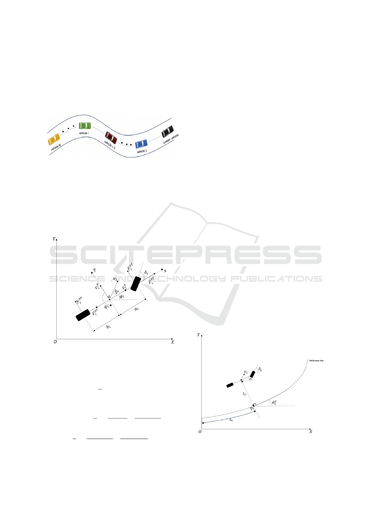
2 VEHICLE PLATOON MODEL

In this paper, as shown in Figure 1, a platoon of vehi-

cles on the curved road is presented, which consists of

a leader vehicle and several following vehicles. The

leader vehicle is denoted as 0, and the following vehi-

cles are denoted as 1 to N, respectively.

Figure 1: Vehicle platoon on the curved road.

2.1 Vehicles Dynamics Model

Since the vehicle platoon in this paper needs to travel

on roads with varying curvature, both lateral and lon-

gitudinal motion control is required. Therefore, as

shown in Figure 2, we introduce a 3-DOF dynamic

bicycle model of the vehicle

Figure 2: 3-DOF dynamic bicycle model of the vehicle.

In Figure 2, X , O, and Y represent the Earth coor-

dinate system, while x, o, and y represent the vehicle

body coordinate system. Based on (Feng et al., 2024),

set u

= ˙v

= v

, we propose a new vehicles

dynamics model which can be expressed as:











˙v

= u

˙v

= −v



−

(

)

−

(

−C

)





−

(

−C

)

−

(

)



(1)

The subscript i denotes the i-th vehicle, where i ∈

{1,2,..., N}. The mass of the i-th vehicle is denoted

by m

. The longitudinal and lateral velocities of the

i-th vehicle are represented by v

and v

, respectively.

The longitudinal forces on the front and rear tires are

denoted by F

and F

, respectively, while the lateral

forces on these tires are denoted by F

and F

. The

moment of inertia of the i-th vehicle about the z-axis

is represented by I

. The distances from the front and

rear axles to the center of mass of the i-th vehicle are

denoted by a

and b

, respectively. The yaw rate of the

i-th vehicle is given by

and C

represent the cornering stiffness of the

front and rear wheels of the vehicle i, respectively.

is the steering angle of the front tires of the i-th

vehicle. u

denotes the acceleration of the i-th vehicle.

2.2 Longitudinal and Lateral Error

Model

Assuming the speed v

and position s

of the leading

vehicle are a priori known, the goal of the following

vehicles is to track the speed of the leading vehicle

while maintaining a desired inter-vehicle distance. In

this paper, the commonly used constant distance pol-

icy is adopted.

For each following vehicle i, i ∈ {1, 2,... ,N}, let

its position be deﬁned as s

. The position error is de-

scribed as:

= s

− s

− i · d

des

(2)

where d

des

represents the desired inter-vehicle dis-

tance, which is a constant.

As shown in Figure 3, the lateral error l

is deﬁned

in the Frenet coordinate system as the distance be-

tween the vehicle’s center of mass and its projection

onto the reference line.

Figure 3: Lateral error in the Frenet coordinate system.

Coupled Lateral and Longitudinal Control for Vehicle Platoons on Curved Roads

287

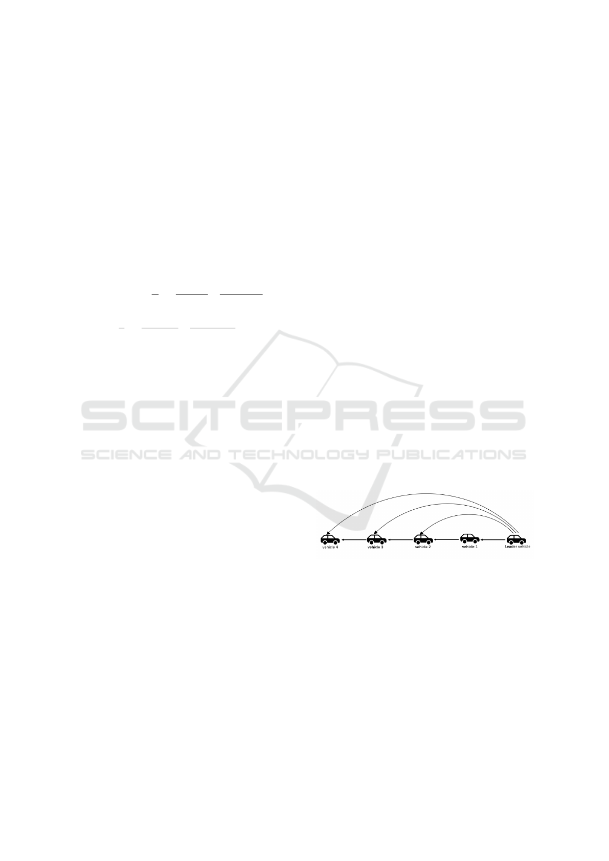
Here, p

is the projection of the center of mass of

vehicle i onto the reference line; v

is the velocity of

the center of mass of vehicle i; ϕ

is the yaw angle of

vehicle i; and θ

is the angle between the tangent to

the reference line at p

and the X-axis. The derivative

of l

with respect to time t is as follows:

= v

cos(ϕ

− θ

) + v

sin(ϕ

− θ

) (3)

2.3 Longitudinal and Lateral Coupled

Model

By combining equations (1), (2), and (3), we obtain

the longitudinal and lateral coupling model for vehi-

cle i:











˙v

= u

˙v

= −v



−

(

)

−

(

−C

)





−

(

−C

)

−

(

)



˙e

= v

− v

= v

cos(ϕ

− θ

) + v

sin(ϕ

− θ

)

(4)

Discretize the system and deﬁne the state variables

as follows:

(k) = [v

(k) v

(k)

(k) ϕ

(k) e

(k) l

(k)]

(5)

The control inputs are the acceleration and the

front wheel steering angle, deﬁned as:

(k) = [u

(k) δ

(k)]

(6)

The output is given by:

(k) = [v

(k) e

(k)]

(7)

Using the Euler forward difference method, the

discrete nonlinear model is given by:

(

(k + 1) = φ



(k),U

(k)



(k) = γX

(k)

(8)

γ =



1 0 0 0 0 0

0 0 0 0 1 0



where γ is the matrix deﬁned above. The function



(k),U

(k)



is speciﬁed in equation (11), and T

represents the discrete time interval.

3 DISTRIBUTED MODEL

PREDICTIVE CONTROL

This section introduces the design of a Distributed

Model Predictive Control (DMPC). Vehicles ex-

change and receive information based on the com-

munication topology. Each vehicle transmits its own

state and the received information to its upper-level

DMPC controller, which then optimizes to compute

the optimal control inputs. The DMPC controller ad-

justs the state of each vehicle to ensure coordinated

behavior of the platoon.

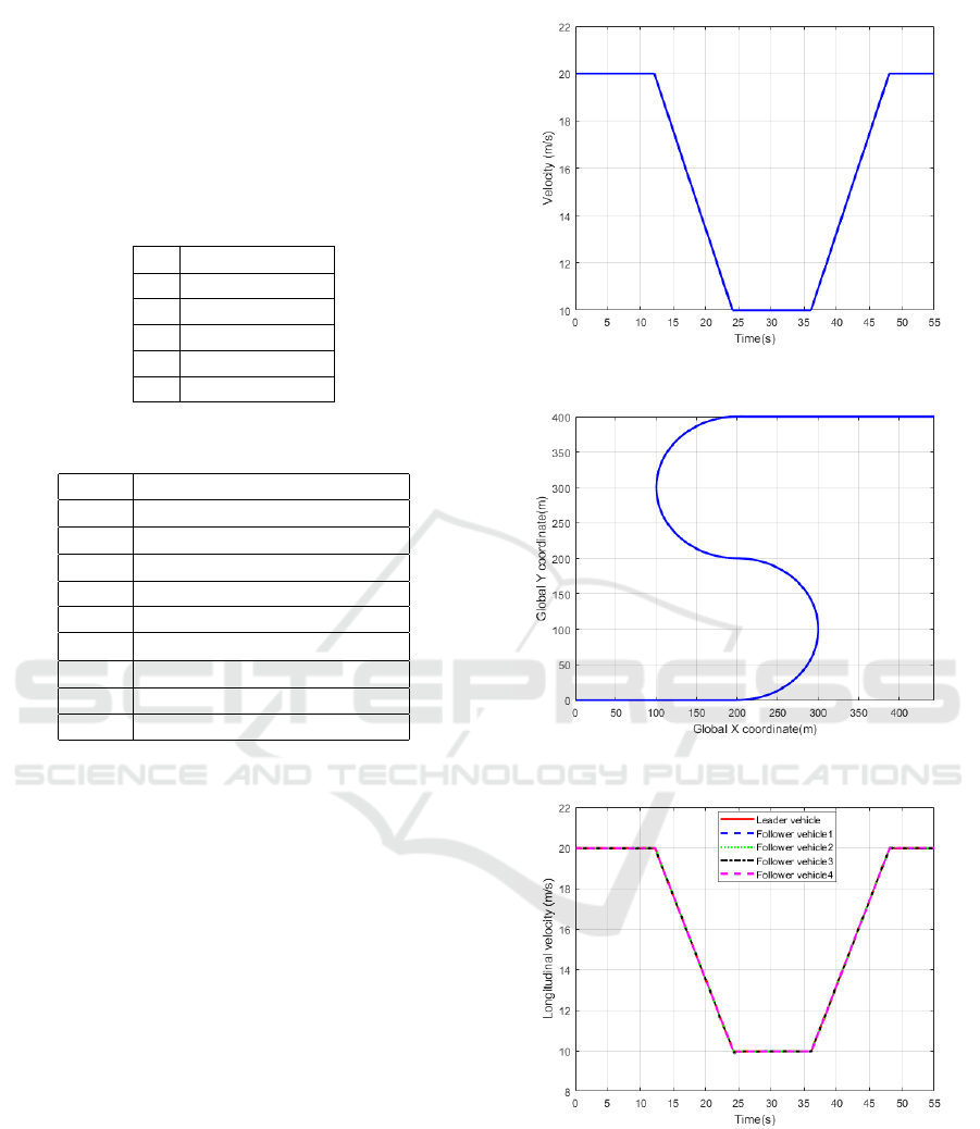
3.1 Communication Topology

The design of the communication topology plays a

crucial role in the formulation of the cost function

in DMPC. The communication topology of the ve-

hicle ﬂeet can be represented by a directed graph

G = {V,E} , where V = {0,1,2, . .., N} is the set of

vehicles, and E ⊆ V × V is the set of edges that con-

nect vehicles, and then deﬁne an N-order real-valued

adjacency matrix A = [a

i j

] ∈ R

N×N

, which is used

to represent the communication relationship between

any two vehicles

A = [a

i j

] =

(

i j

= 1, if

{

j, i

}

∈ E

i j

= 0, if

{

j, i

}

/∈ E

(10)

where i, j ∈ V and { j,i} ∈ E indicate a directed edge

from j to i, meaning that information from vehicle j

can be transmitted to vehicle i. We deﬁne N

= { j |

i j

= 1, j ∈ {1,2, . .., N}} as the neighbor set of ve-

hicle i, which implies that vehicle i can receive infor-

mation from any vehicle j ∈ N

. Similarly, we deﬁne

= { j | a

= 1, j ∈ {1,2, ..., N}}, representing the

set of vehicles to which vehicle i can transmit infor-

mation. In this paper, we adopt the commonly used

predecessor-leader following (PLF) topology, as illus-

trated in Figure 4.

Figure 4: Predecessor-leader following (PLF) topology.

3.2 Controller Design

DMPC transforms the global problem into a local

problem for each vehicle, where all vehicles simul-

taneously solve their own optimization problems.

Assume that the lead vehicle is not controlled and

always follows the ideal trajectory. Then, accord-

ing to equation (7), we deﬁne the reference values

i,des

(k) for the follower vehicles in the platoon:

i,des

(k) =

i,des

(k) v

i,des

(k)

i,des

(k) ϕ

i,des

(k) e

i,des

(k) l

i,des

(k)]

(11)

where v

i,des

(k) is the desired speed of vehicle i.

VEHITS 2025 - 11th International Conference on Vehicle Technology and Intelligent Transport Systems

288



(k),U

(k)









(k)T

+ v

(k)

−v

(k)

(k) +

−

(k)

−

−C

)

(k)

+ v

(k)

−

−C

(k)

−

)

(k)

(k)T

+ ϕ

(k)

(k) − v

(k)) T

+ e

(k)



(k) cos



(k) − θ

(k)



+ v

(k) sin



(k) − θ

(k)



+ l

(k)







(9)

In the platoon, the desired speed of the follower

vehicles should track the speed of the lead vehicle,

thus let v

i,des

(k) = v

(k). The desired lateral speed

i,des

(k) = 0, but this does not mean that we expect

the lateral speed to be exactly zero, as it is impossible

for the vehicle’s lateral speed to be zero when driving

through a curve. We simply want the lateral speed to

be as small as possible to reduce vehicle oscillation.

Assuming that the onboard equipment can mea-

sure the road radius R, meaning the road radius is

known, then the ideal yaw rate is:

i,des

(k) =

(k)

. (12)

The ideal yaw angle, as shown in Figure 3, is

the angle between the tangent to the reference line at

point p

and the X-axis, i.e.,

i,des

(k) = θ

(k). (13)

The ideal spacing error e

i,des

(k) = 0 and the ideal

lateral distance error l

i,des

(k) = 0, as we want to main-

tain a safe set distance between vehicles and ensure

that each following vehicle travels along the reference

line.

In the local problem for each following vehicle,

deﬁne the same prediction horizon N

. In the pre-

diction horizon [k, k + N

], three state trajectories are

deﬁned.

1) X

(t|k) : Predicted state trajectory.

(t|k) : Assumed state trajectory.

3) X

∗

(t|k) : Optimal state trajectory.

Here, t = 0,1, . .., N

. Similarly, deﬁne three con-

trol input trajectories.

1) U

(t|k) : Predicted control input trajectory.

(t|k) : Assumed control input trajectory.

3) U

∗

(t|k) : Optimal control input trajectory.

Within the prediction horizon, deﬁne the reference

state trajectory

i,des

(t|k) =

i,des

(t|k) v

i,des

(t|k)

i,des

(t|k) ϕ

i,des

(t|k)

i,des

(t|k) l

i,des

(t|k)]

(14)











i,des

(t|k) = v

(k)

i,des

(t|k) = 0

i,des

(t|k) =

˜v

(t|k)

i,des

(t|k) = θ

(t|k)

i,des

(t|k) = 0

i,des

(t|k) = 0

t = 0,1, ...,N

(15)

where ˜v

(t|k) is the ﬁrst term in the assumed state tra-

jectory, and θ

(t|k) can be computed from the refer-

ence line information collected by the onboard equip-

ment.

Now, we present the local optimization control

problem for each vehicle i .

Problem P : For each vehicle i, i ∈ 1, 2, ... , N, at

time k

min

(:|k)

−1

∑

t=0



(t|k),y

(t|k), ˜y

(t|k),U

(t|k)





|k) − X

i,des

|k)



(16a)

subject to

(t + 1|k) = φ



(t|k),U

(t|k)



(t|k) = γX

(t|k)

(0|k) = X

(k)

(16b)

i,min

≤ u

a,p

(t|k) ≤ u

i,max

(16c)

i,min

≤ δ

(t|k) ≤ δ

i,max

(16d)

Coupled Lateral and Longitudinal Control for Vehicle Platoons on Curved Roads

289

where



(t|k),y

(t|k), ˜y

(t|k),U

(t|k)





(t|k) − X

i,des

(t|k)



(t|k) − ˜y

(t|k)



∑

j∈N



(t|k) − ˜y

(t|k)



(t|k)



(17)

where U

(: |k) = [U

(0|k),... ,U

− 1|k)] repre-

sents the unknown control input trajectory to be op-

timized, Q

∈ S

, F

∈ S

, M

∈ S

, R

∈ S

are the

weighting matrices and they are all symmetric pos-

itive deﬁnite matrices.

∥

represents

∥

o. ˜y

(t|k) = γ

(t|k) is the assumed output of the

vehicle i, and ˜y

(t|k) = γ

(t|k) is the assumed output

of the neighboring vehicle j of the vehicle i. (16c)

and (16d) represent constraints on the control inputs

of acceleration and front wheel steering angle, ensur-

ing that the vehicle’s acceleration, deceleration, and

front wheel steering angles remain within the physi-

cally feasible limits.

In the cost function (17)



(t|k) − X

i,des

(t|k)



represents the penalty

for the error between the predicted state trajectory of

vehicle i and the desired state trajectory.



(t|k) − ˜y

(t|k)



represents the penalty for

the error between the predicted output trajectory of

vehicle i and the assumed output trajectory.

3) ∥y

(t|k) − ˜y

(t|k)∥

represents the penalty for

the error between the predicted output trajectory of

vehicle i and the assumed output trajectory vehicle j.



(t|k)



represents the penalty for the con-

trol inputs of acceleration and front wheel steering an-

gle for vehicle i .

Furthermore,



|k) − X

i,des

|k)



is the

terminal cost function.

3.3 Algorithm of DMPC

The assumed control input trajectory

(t|k) is iter-

ated using the following equation

(t|k) =

(

∗

(t + 1|k − 1),t = 0, 1,...,N

− 2

∗

− 1|k − 1),t = N

− 1

(18)

The assumed state trajectory

(t|k) is then com-

puted based on the assumed control input trajectory

(t + 1|k) = φ



(t|k),

(t|k)



(0|k) = X

∗

(1|k − 1)

˜y

(t|k) = γ

(t|k)

t = 0,1, ...,N

− 1

(19)

The DMPC algorithm is presented as Algorithm 1:

Algorithm 1: DMPC Algorithm.

1 Initialization:

/* At time k =0, initialize the

assumed state trajectory for

vehicle i = 1,2, ...,N. */

2 Initialize the state variables X

(0) and control

inputs U

(0) of vehicle i.

(t|0) = U

(0),t = 0,1,...,N

;

4 for t = 0 to N

− 1 do

(t + 1|0) = φ



(t|0),

(t|0)



;

6 ˜y

(t|0) = γ

(t|0);

(0|0) = X

(0);

8 end

9 Iteration:

/* At time k>0, all vehicles

i = 1,2, ...,N perform iterative

computations. */

10 while the lead vehicle has not stopped do

11 1) Vehicle i gets the optimal control input

trajectory U

∗

(t|k) through solving the

problem P ;

12 2) Calculate the optimal state trajectory.

13 for t = 0 to N

− 1 do

14 X

∗

(t + 1|k) = φ

∗

(t|k),U

∗

(t|k));

15 X

∗

(0|k) = X

(k);

16 end

17 3) Calculate the assumed control and

output trajectories for the next time step

using equations (18) and (19);

18 4) Transmit ˜y

(t|k + 1) to vehicles j ∈ O

receive ˜y

(t|k + 1) from vehicles j ∈ Ni,

and obtain Xi,des(t|k + 1) from the lead

vehicle and onboard systems;

19 5) Apply the ﬁrst element of the optimal

control input, U

(t) = U

∗

(0|k), to

vehicle i;

20 6) Set k = k + 1;

21 end

Algorithm 1 presents the detailed steps of the

DMPC algorithm. Within this framework, each ve-

hicle in the ﬂeet simultaneously solves its own opti-

mization problem. This synchronized execution en-

sures the effectiveness of real-time control.

4 SIMULATION

The simulation will use CarSim 2016 and Matlab

2020b in conjunction. We validate the effectiveness

of the longitudinal and lateral coupling platoon con-

trol model.

VEHITS 2025 - 11th International Conference on Vehicle Technology and Intelligent Transport Systems

290

4.1 Parameter Settings

In this section, we will provide information about the

vehicle and relevant parameters in the control algo-

rithm. The vehicles in the simulation are homoge-

neous. The parameter settings can be found in Table

1 and Table 2.

Table 1: Vehicle parameters.

110000(N/rad)

1.015(m)

1.950(m)

1412(kg)

1536.7(kg·m²)

Table 2: Control parameters.

diag(5, 1, 5, 500, 10, 10)

diag(1, 100)

diag(10, 10)

0.1(s)

i,min

-8(m/s²)

i,max

5(m/s²)

i,min

-1(rad)

i,max

1(rad)

4.2 Simulation Results

This case is used to verify the effectiveness of the lon-

gitudinal and lateral coupling platoon control model

proposed in this paper.

Set the initial position of the lead vehicle s

60m, the initial position of the following vehicle s

45m, s

= 30m, s

= 15m, s

= 0m. Set the desired

inter-vehicle distance as d

des

= 15m. The velocity tra-

jectory of the lead vehicle is shown in Figure 5. The

reference line is shown in Figure 6.

The simulation results are shown from Figures 7

to 10. Figure 7 presents the vehicle velocities. It

can be observed that the following vehicles in the pla-

toon closely track the lead vehicle’s speed during con-

stant, deceleration, and acceleration phases. Figure 8

shows the vehicle positions, demonstrating that safe

distances between vehicles are maintained throughout

the simulation, preventing collisions. Figure 9 illus-

trates the ideal inter-vehicle spacing errors. Under the

PLF topology, since the ﬁrst following vehicle only

receives information from the lead vehicle, its reac-

tion is more intense when the lead vehicle changes

speed, resulting in relatively larger spacing errors. In

Figure 5: Lead vehicle’s desired velocity trajectory.

Figure 6: Reference line.

Figure 7: Velocity of vehicles.

contrast, the following vehicles can receive informa-

tion from both the lead vehicle and the preceding ve-

hicle, which leads to smaller spacing errors. Overall,

the spacing errors between vehicles remain within a

small range. Figure 10 illustrates the lateral distance

error of the vehicles. It shows that the lateral distance

error is minimal, indicating that the vehicles main-

Coupled Lateral and Longitudinal Control for Vehicle Platoons on Curved Roads

291

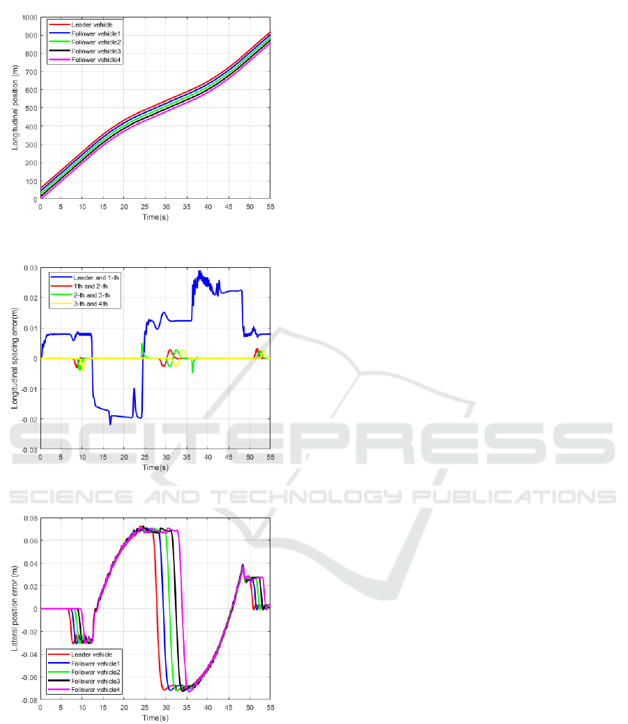
Figure 8: Longitudinal position of vehicles.

Figure 9: Longitudinal spacing error.

Figure 10: Lateral position error.

tain excellent lane-keeping performance while driving

on roads with varying curvature, avoiding the cutting-

corner problem and preventing drifting out of lane.

5 CONCLUSION

This paper focuses on platoon driving on curved

roads by integrating a 3-DOF dynamic vehicle model

with lateral distance in the Frenet coordinate sys-

tem, forming a new longitudinal and lateral cou-

pled platoon control model, which is controlled by

DMPC (Distributed Model Predictive Control). Sim-

ulations demonstrate the good performance of the

longitudinal-lateral coupled platoon control model. In

the future, we plan to extend our research to cooper-

ative control among more platoons, such as two or

three platoons, and explore better models to improve

control performance.

ACKNOWLEDGEMENTS

This work is supported by Zhejiang Provincial

Natural Science Foundation of China (Grant No.

LQ23F030014), National Natural Science Foundation

of China (Grant No. 62303410), and Open Research

Project of State Key Laboratory of Industrial Control

Technology, Zhejiang University, China (Grant No.

ICT2024B46).

REFERENCES

Basiri, M. H., Ghojogh, B., Azad, N. L., Fischmeister, S.,

Karray, F., and Crowley, M. (2020). Distributed non-

linear model predictive control and metric learning for

heterogeneous vehicle platooning with cut-in/cut-out

maneuvers. In 2020 59th IEEE Conference on Deci-

sion and Control (CDC), pages 2849–2856.

Bayuwindra, A., Ploeg, J., Lefeber, E., and Nijmeijer, H.

(2020). Combined longitudinal and lateral control of

car-like vehicle platooning with extended look-ahead.

IEEE Transactions on Control Systems Technology,

28(3):790–803.

Dai, Y., Yang, Y., Wang, Z., and Luo, Y. (2022). Exploring

the impact of damping on connected and autonomous

vehicle platoon safety with cacc. Physica A: Statisti-

cal Mechanics and its Applications, 607:128181.

Dunbar, W. B. and Caveney, D. S. (2012). Distributed re-

ceding horizon control of vehicle platoons: Stability

and string stability. IEEE Transactions on Automatic

Control, 57(3):620–633.

Feng, Y., Yu, S., Sheng, E., Li, Y., Shi, S., Yu, J., and

Chen, H. (2024). Distributed mpc of vehicle platoons

considering longitudinal and lateral coupling. IEEE

Transactions on Intelligent Transportation Systems,

25(3):2293–2310.

He, J., Zhao, F., Zhu, S., Li, S., and Xu, J. (2024). Priority-

based deadlock recovery for distributed swarm ob-

stacle avoidance in cluttered environments. In 2024

VEHITS 2025 - 11th International Conference on Vehicle Technology and Intelligent Transport Systems

292

IEEE/RSJ International Conference on Intelligent

Robots and Systems (IROS), pages 14056–14062.

IEEE.

Kianfar, R., Ali, M., Falcone, P., and Fredriksson, J. (2014).

Combined longitudinal and lateral control design for

string stable vehicle platooning within a designated

lane. In 17th International IEEE Conference on In-

telligent Transportation Systems (ITSC), pages 1003–

1008.

Kwon, J.-W. and Chwa, D. (2014). Adaptive bidirectional

platoon control using a coupled sliding mode control

method. IEEE Transactions on Intelligent Transporta-

tion Systems, 15(5):2040–2048.

Li, S. E., Zheng, Y., Li, K., Wu, Y., Hedrick, J. K., Gao,

F., and Zhang, H. (2017). Dynamical modeling and

distributed control of connected and automated vehi-

cles: Challenges and opportunities. IEEE Intelligent

Transportation Systems Magazine, 9(3):46–58.

Ma, K., Wang, H., and Ruan, T. (2021). Analysis of road

capacity and pollutant emissions: Impacts of con-

nected and automated vehicle platoons on trafﬁc ﬂow.

Physica A: Statistical Mechanics and its Applications,

583:126301.

Negenborn, R. and Maestre, J. (2014). Distributed model

predictive control: An overview and roadmap of fu-

ture research opportunities. IEEE Control Systems

Magazine, 34(4):87–97.

Rajamani, R., Tan, H.-S., Law, B. K., and Zhang, W.-B.

(2000). Demonstration of integrated longitudinal and

lateral control for the operation of automated vehicles

in platoons. IEEE Transactions on Control Systems

Technology, 8(4):695–708.

Wei, S., Zou, Y., Zhang, X., Zhang, T., and Li, X. (2019).

An integrated longitudinal and lateral vehicle follow-

ing control system with radar and vehicle-to-vehicle

communication. IEEE Transactions on Vehicular

Technology, 68(2):1116–1127.

Wu, J., Wang, Y., and Yin, C. (2022). Curvilinear multi-

lane merging and platooning with bounded control in

curved road coordinates. IEEE Transactions on Vehic-

ular Technology, 71(2):1237–1252.

Zeng, J., Qian, Y., Li, J., Zhang, Y., and Xu, D. (2023).

Congestion and energy consumption of heterogeneous

trafﬁc ﬂow mixed with intelligent connected vehicles

and platoons. Physica A: Statistical Mechanics and its

Applications, 609:128331.

Zhao, H., Sun, D., Zhao, M., Pu, Q., and Tang, C. (2022).

Combined longitudinal and lateral control for hetero-

geneous nodes in mixed vehicle platoon under v2i

communication. IEEE Transactions on Intelligent

Transportation Systems, 23(7):6751–6765.

Zheng, Y., Li, S. E., Li, K., Borrelli, F., and Hedrick,

J. K. (2017). Distributed model predictive control for

heterogeneous vehicle platoons under unidirectional

topologies. IEEE Transactions on Control Systems

Technology, 25(3):899–910.

Zuo, Z., Yang, K., Wang, H., Wang, Y., and Wu, Y. (2024).

Distributed mpc for automated vehicle platoon: A

path-coupled extended look-ahead approach. IEEE

Transactions on Intelligent Vehicles, pages 1–13.

Coupled Lateral and Longitudinal Control for Vehicle Platoons on Curved Roads

293