LIC-R: Line Integral Convolution Revisited
Khatereh Mohammadi
a
, Marco Agus
b
, Ahmad Abushaikha
c
and Jens Schneider
d
College of Science and Engineering, Hamad Bin Khalifa University, Doha, Qatar
Keywords:
Line Integral Convolution, Flow Visualization, Eulerian Formulations.
Abstract:
We present a novel formulation of Line Integral Convolution (LIC), a fundamental method for visualizing
vector fields in flow visualization. Our approach reinterprets the traditional LIC technique by leveraging a
regularized, directional curvature flow along streamlines, utilizing material derivatives to achieve the desired
convolution. By adopting an entirely Eulerian framework, our method eliminates the need for complex numer-
ical integration and high-order interpolation schemes that are typically required in classical LIC algorithms.
This shift not only simplifies the implementation of LIC, making it more accessible for both CPU and GPU
architectures, but also significantly reduces the computational overhead. Despite these simplifications, our
method maintains visual quality comparable to that of more traditional and computationally expensive ap-
proaches. Moreover, the discrete nature of our formulation makes it particularly well-suited for irregular grids
and sparse data, broadening its applicability in practical settings. Through various experiments, we demon-
strate that our algorithm delivers efficient and visually coherent results, offering an attractive alternative for
dense flow visualization with reduced complexity.
1 INTRODUCTION
Flow visualization is a crucial area of scientific visu-
alization focused on representing vector fields—such
as fluid motion, air currents, or magnetic fields—in
a way that makes their structure and dynamics visu-
ally understandable. By enabling the study of pat-
terns like vortices, divergences, and flow separations,
flow visualization is widely used in various fields, in-
cluding fluid dynamics, meteorology, medical imag-
ing, and aerodynamics (Delmarcelle and Hesselink,
2023). Accurate and efficient visualization of flow
data is essential for understanding complex behav-
iors in natural and engineered systems, helping sci-
entists and engineers in tasks ranging from analyz-
ing weather patterns to optimizing the performance
of mechanical components (Yau, 2024).
2023 marked the 30
th
anniversary of the Line In-
tegral Convolution (LIC) method. Since its incep-
tion by (Cabral and Leedom, 1993), LIC has become
one of the most popular and widely adopted tech-
niques for dense and continuous visualization of vec-
tor fields. This method has been particularly valued
a
https://orcid.org/0009-0008-2636-8053
b
https://orcid.org/0000-0003-2752-3525
c
https://orcid.org/0000-0002-6916-050X
d
https://orcid.org/0000-0003-4751-9152
for its ability to generate high-quality visualizations
of flow data. Over the past three decades, several im-
provements and variations of the LIC algorithm have
been proposed to address its limitations and enhance
its capabilities (Stalling and Hege, 1995; Laramee
et al., 2008; Weinkauf and Theisel, 2010), solidify-
ing its position as a go-to tool in flow visualization.
The classical LIC algorithm is conceptually
simple, which is one of its key strengths. It begins
with a random image I : Ω → [0,1], where Ω is a d-
dimensional domain, and a vector field V : Ω → R
d
,
defined over the same domain. The fundamental idea
is to compute streamlines, which are curves that are
everywhere tangential to the vector field V, passing
through each pixel of the image. Once streamlines
are generated, the image I is filtered along these
streamlines using a low-pass convolution kernel.
This process results in strong spatial coherence along
the streamlines (i.e., along the flow direction) and
reduced coherence across (i.e., perpendicular to the
flow), producing the familiar streaked appearance
characteristic of LIC visualizations. Traditionally,
LIC is computed on a grayscale image, with color
often reserved as an additional channel to encode
other data properties. Figure 1 provides an illustrative
example of such an LIC visualization.
Mohammadi, K., Agus, M., Abushaikha, A. and Schneider, J.
LIC-R: Line Integral Convolution Revisited.
DOI: 10.5220/0013131700003912
Paper published under CC license (CC BY-NC-ND 4.0)
In Proceedings of the 20th International Joint Conference on Computer Vision, Imaging and Computer Graphics Theory and Applications (VISIGRAPP 2025) - Volume 1: GRAPP, HUCAPP
and IVAPP, pages 875-886
ISBN: 978-989-758-728-3; ISSN: 2184-4321
Proceedings Copyright © 2025 by SCITEPRESS – Science and Technology Publications, Lda.
875

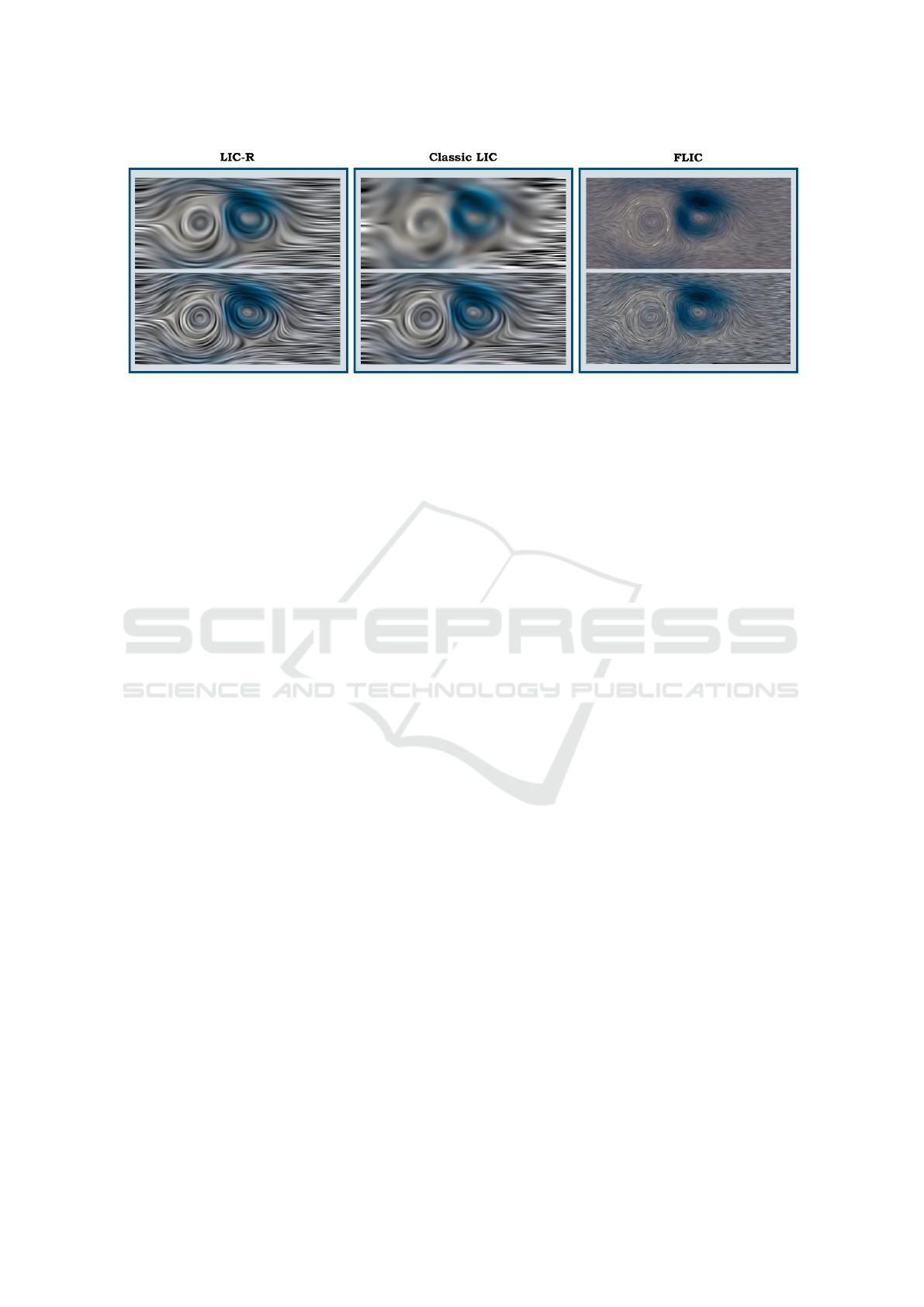
Figure 1: We present LIC-R, a novel efficient formulation for line integral convolution taking inspiration from the material
derivative from continuum mechanics. Our method is able to capture the main features of flows with a quality comparable to
classic LIC and fast LIC computed using high-order sampling and integration schemes but is significantly faster than classic
LIC (up to one order of magnitude) and achieves better quality than Fast LIC with comparable processing times. In the
example above, a frame from jungtelziemniak simulation.
Despite its effectiveness, the classical LIC ap-
proach has several challenges and shortcomings. One
significant issue is that the vector field is often avail-
able only at discrete sampling points, particularly
when working with real-world or simulated data. To
address this, LIC requires interpolation schemes to re-
construct the continuous vector field V from these
discrete samples. The choice of interpolation can
have a large impact on the quality of the resulting
visualization. For high-quality LIC images, higher-
order interpolation schemes, such as cubic Catmull-
Rom splines (Catmull and Rom, 1974), are frequently
employed. However, this introduces additional com-
putational complexity.
Another challenge arises from the need to com-
pute streamlines through numerical integration. The
accuracy and smoothness of the streamlines are also
highly dependent on the integrator used. High-order
numerical integration schemes, such as the classical
fourth-order Runge-Kutta method (Stalling, 1998),
are often required for high-quality results. These
higher-order methods, while effective, introduce
significant computational overhead and complexity,
both in terms of implementation and performance.
Thus, while the original LIC algorithm is conceptu-
ally straightforward, its practical implementation can
become quite intricate and computationally expensive
due to the necessity of high-order interpolation and
integration methods.
As a result, implementing classical LIC remains
a complex and resource-intensive task rooted in the
Lagrangian view of flow, which requires tracing
individual particle paths through a continuous vector
field. The reliance on this Lagrangian approach
necessitates careful balancing of accuracy, com-
putational cost, and visual quality, often requiring
trade-offs based on the specific application. Addi-
tionally, the need for high-order interpolation and
integration makes the method less suited for real-time
applications or situations where computational
resources are limited.
Contributions. In this paper, we propose a novel
approach to LIC that shifts away from the traditional
Lagrangian view and adopts a fully Eulerian perspec-
tive. Rather than interpolating the vector field to re-
construct continuous flow paths, we work directly
with the discrete vector samples. This shift allows
us to reinterpret the LIC process as a discrete cur-
vature flow along each streamline, using directional
derivatives that naturally align with the parametric
derivatives of traditional LIC. Our formulation not
only simplifies the implementation but also signifi-
cantly reduces computational costs by avoiding the
need for high-order interpolation and numerical in-
tegration. Importantly, our method produces visual
results that are comparable in quality to much more
computationally expensive approaches.
Furthermore, since our technique does not rely on
interpolation to a continuum, it is easily generalized
to vector fields that are sampled on irregular grids,
broadening the potential application of LIC to a wider
range of data sources. This paper provides a detailed
discussion of our novel formulation and demonstrates
its effectiveness across several different test cases.
Organization. The remainder of this paper is struc-
tured as follows: In the next section, we review
related work, focusing on major improvements and
variations of the original LIC algorithm that have
IVAPP 2025 - 16th International Conference on Information Visualization Theory and Applications
876

been proposed over the past 31 years. Section 3 pro-
vides the mathematical foundations of our new Eu-
lerian LIC approach, including the re-derivation of
the LIC process using discrete curvature flow. Sec-
tion 4 details the implementation of our algorithm and
highlights its computational advantages. Finally, we
present results and discuss limitations in Section 5,
before concluding the paper with an outlook on future
work.
2 RELATED WORK
Our method deals with image-based visualization of
vector fields. Such fields have attracted the atten-
tion of the visualization community for a long time
and we do not aim to provide a comprehensive dis-
cussion of the impressive body of relevant literature.
Instead, we refer the reader to (Laramee et al., 2008)
excellent survey on texture-based flow visualization
as well as more recent surveys covering flow visual-
ization for environmental science (Bujack and Mid-
del, 2020), state-of-the-art methods for vortex extrac-
tion (G
¨
unther and Theisel, 2018), and time-dependent
flow topology (Bujack et al., 2020).
Recent trends in flow visualization (G
¨
unther,
2020) are targeting the challenges related to automatic
extraction and visual analysis of vortices and flow
features by considering observer-relative frame ref-
erences (Hadwiger et al., 2019; Rautek et al., 2021;
G
¨
unther et al., 2017; Zhang et al., 2022; G
¨
unther and
Theisel, 2024) or topology-based methods (Rojo and
G
¨
unther, 2020; Hofmann and Sadlo, 2021). To this
end, the community has started to explore modern
machine learning, for example for performing neural
flow map interpolation (Jakob et al., 2021), or for au-
tomatic extraction of reference frames through con-
volutional neural networks (Kim and G
¨
unther, 2019).
Very recently, (Daßler and G
¨
unther, 2024) defined
a theoretical framework for extracting flow features
through variational methods.
In the following, we discuss the classical image-
based methods most closely related to our formula-
tion. Since the publication of (Cabral and Leedom,
1993) seminal paper, the visualization community di-
rected massive efforts to improve the original formu-
lation and to apply it to a variety of scientific domains.
The original method basically involves the convolu-
tion of a noise texture with a kernel function along a
characteristic path defined by the flow field in a way
to produce a streaky visualization that highlights the
structure of the flow and allows for immediate under-
standing of its features.
(Rezk-Salama et al., 1999) extended the formu-
lation to 2D surfaces through the usage 3D tex-
tures, (Stalling and Hege, 1995) derived a resolution-
independent formulation that also addresses the orig-
inal LIC’s high computational demands, (Wegenkittl
et al., 1997) extended the original formulation to
asymmetric kernels to generate oriented patterns that
are able to highlight the flow orientation, (Forsell
and Cohen, 1995) extended LIC to curvilinear grids,
while (Sundquist, 2003) proposed a dynamic version
for representing streamline evolution. LIC on sur-
faces is also discussed thoroughly in (Stalling, 1998)
PhD thesis, as is the numerical machinery for that pur-
pose. To address the computational cost of 3D LIC
and surface LIC, image-based computation has been
proposed (van Wijk, 2003; Telea and van Wijk, 2003)
but the resulting visualization is not frame-coherent
in animations.
Concerning the various applications, apart of di-
rect visualization of flows for environmental sci-
ences and engineering (Bujack and Middel, 2020),
the method has been successfully applied in geom-
etry processing for effective illustration of surface
shapes (Interrante, 1997), for highlighting the salient
regions in molecular surfaces (Lawonn et al., 2014),
for terrain and cartography applications (Jenny,
2021), and for highlighting fiber tracts maps from dif-
fusion tensor imaging (McGraw et al., 2002). Very
recently, (Rautek et al., 2023) integrated line inte-
gral convolution in a framework for interactive anal-
ysis and identification of physically observable vor-
tex structures. Inspired by advection and the con-
cept of the material derivative in continuum mechan-
ics, which refers to the rate of change over time of
a physical quantity in a material element exposed to
a velocity field (Sun, 2020), we propose a novel Eu-
lerian formulation for line integral convolution. Our
method is based on the material transport of underly-
ing noise images. Eulerian formulations are popular
for computing and rendering Finite-Time Lyapunov
Exponents to characterize coherent Lagrangian struc-
tures (Garth et al., 2007; Sadlo and Peikert, 2007),
or for performing post-hoc flow analysis (Agranovsky
et al., 2014). (Hanser et al., 2019) recently also con-
sidered the material derivative concept for creating
an energy-based visual analysis system for 2D flow
fields.
3 METHODOLOGY
In this section, we detail our novel approach for com-
puting Line Integral Convolution (LIC) using a reg-
ularized, directional curvature flow along streamlines
in the vector field. Our method builds upon the clas-
LIC-R: Line Integral Convolution Revisited
877

sical LIC framework but simplifies the computation
by eliminating the need for interpolation and numer-
ical integration. Below is a brief outline of the key
components:
• Continuum Formulation. We begin with the
classical definition of LIC using streamlines and
arc-length parameterization. Our method adapts
this to directional derivatives along the vector
field, allowing for efficient computation.
• Material Derivative and Curvature Flow. In-
stead of advection, we introduce a curvature-
based flow derived from the second order direc-
tional derivative, analogous to the material deriva-
tive in fluid dynamics (Sun, 2020).
• Discrete Setting. The vector field and image
are discretized on a grid, and we derive second
and fourth order difference stencils for directional
derivatives to efficiently compute the LIC result
on both uniform and irregular grids.
• Numerical Solution. We present an iterative
numerical solution using Gauss-Seidel steps for
solving the resulting system matrix. The full so-
lution is obtained by combining equilibrium and
perturbed step solutions.
3.1 Continuum Formulation
Given a d−dimensional vector field V : Ω → R
d
over
a domain Ω ⊆ R
d
, streamlines are defined as lines
tangential to V. Given a point x
0
∈ Ω, individual
streamlines passing through x
0
can be computed ex-
plicitly by forward and backward integration, result-
ing in positions p(x
0
,t) along a curve parameterized
by t. From the definition it is clear that the result-
ing curve is Euler-invariant, that is, p(x
0
,t) does not
change under different parameterizations. LIC uses
this fact to extract curves under an arc-length param-
eterization s, p(x
0
,s), for which
dp
ds
=
V (p(s))
∥
V (p(s))
∥
2
. (1)
LIC uses these streamlines to convolve a low-pass fil-
ter κ of length L with an image I containing uncorre-
lated noise, to compute the final image L,
L(x
0
) =
Z
L/2
−L/2
κ(s)I (p(x
0
,s))ds. (2)
Our approach, in contrast, uses Eqn. (1) to define
directional derivatives:
dp
ds
=
∂p
∂v
, (3)
where v is a normalized (unit) vector of the underly-
ing vector field. Using the chain rule, we have
∂p
∂v
=
∂p
∂x
∂x
∂v
. (4)
The term ∂x/∂v in Eqn. (4) measures the change of
x in direction of v, which is equivalent to the compo-
nents of v. We thus obtain
∂p
∂v
=
⟨
v, ∇p
⟩
. (5)
For the secondorder derivative, we analogously use
∂
2
p
∂v
2
= v
T
H
p
v, (6)
where H
p
is the Hessian of p.
3.2 Material Derivative and Curvature
Flow
Computing ∇p and H
p
seems problematic at
first glance, since each individual path should be
paremetrized and the notion of a canonical coordinate
frame x changes along the path p. It is at this point
where we take inspiration from the material deriva-
tive. Given a material field I(x,t) and a macroscopic
velocity field (one that depends only on space-time)
v(x,t), the material derivative measures total change
over time. It is defined as
DI
Dt
:=
∂I
∂t
+
⟨
v , I
⟩
. (7)
The two terms in Eqn. 7 model the change in ma-
terial due to external (∂I/∂t) and advection effects
(⟨v , I⟩), introducing an artificial integration time pa-
rameter t even for stationary fields. In our case, the
first term vanishes. Since we are not interested in ad-
vecting the material but rather smoothing along each
streamline, we define a material curvature, using the
second order directional derivative instead, resulting
in the following curvature flow.
DI
Dt
:=




∂
2
I
∂v
2




. (8)
This gives rise to a sequence of images I(x,t) that is
now decoupled from the underlying streamlines. Note
that the 2
nd
order directional derivative is equivalent
to a derivative with respect to arc-length and, thus,
its modulus measures the curvature (Farin, 2001) of
the image in direction v. Note that in our use case,
an arclength parameterization of characteristic curves
can be obtained by pre-normalizing the vector field,
except for stationary points which should remain at
0-magnitude (see also Sec. 4 on stationary points).
IVAPP 2025 - 16th International Conference on Information Visualization Theory and Applications
878

Table 1: Components of the central difference stencils (cf. (12)) used in this work. Adding the stencils in either the O

∆x
2

or O

∆x
4

columns yields 2
nd
or 4
th
-order discretisations of the second directional derivative with respect to v = (v
1
,v
2
).
The velocity v is sampled at the center of the stencil.
∂
2
∂v
2
O

∆x
2

O

∆x
4

∂
2
∂x
2
1
1
∆x
1


0 0 0
1 −2 1
0 0 0


v
1
12∆x
2
1





0 0 0 0 0
0 0 0 0 0
−1 16 −30 16 −1
0 0 0 0 0
0 0 0 0 0





∂
2
∂x
2
2
1
∆x
2


0 1 0
0 −2 0
0 1 0


v
1
12∆x
2
2





0 0 −1 0 0
0 0 16 0 0
0 0 −30 0 0
0 0 16 0 0
0 0 −1 0 0





∂
2
∂x
1
∂x
2
1
4∆x
1
∆x
2


1 0 −1
0 0 0
−1 0 1


v
1
v
2
72∆x
1
∆x
2





1 −8 0 8 −1
−8 64 0 −64 8
0 0 0 0 0
8 −64 0 64 −8
−1 8 0 −8 1





3.3 Discrete Setting
For the sake of clarity, we assume for now that both
the vector field V and the image I are sampled on
a uniform 2D grid. However, neither dimension
nor uniformity of the grid are a requirement of our
method. To discretize Eqn. (8) we use discrete dif-
ferences. We consider both second order and fourth
order stencils, which can be derived in the classical
fashion (i.e., using a Taylor expansion around any
grid point). Expanding the second order derivative in
Eqn. (8) using the formulation in Eqn. (6), we obtain
∂
2
I
∂v
= v
2
1
∂
2
I
∂x
2
1
+ v
2
2
∂
2
I
∂x
2
2
+ 2v
1
v
2
∂
2
I
∂x
1
∂x
2
, (9)
where subscripts denote vector components. The sec-
ond order discrete difference stencils are
∂
2
∂x
2
=
1
∆x
2

1 −2 1

+ O

∆x
2

and
∂
∂x
=
1
2∆x

−1 0 1

+ O

∆x
2

. (10)
The fourth order counterparts are
∂
2
∂x
2
=
1
12∆x
2

−1 16 −30 16 −1

+ O

∆x
4

and (11)
∂
∂x
1
=
1
12∆x

1 −8 0 8 −1

+ O

∆x
4

.
Combining these stencils along directions x
1
,x
2
and assuming unit ∆x, we assemble 2D stencils (3×3
and 5 × 5, respectively) for the second order direc-
tional derivative (⊗ denotes an exterior vector prod-
uct, interpreting vectors as matrices and giving rise to
a matrix),
∂
2
∂v
2
= v
2
1
∂
2
∂x
2
1
+ v
2
2

∂
2
∂x
2
2

T
+ 2v
1
v
2
∂
∂x
1
⊗

∂
∂x
2

T
,
(12)
that takes a form of a matrix with circulant-like
structure, that in the following we will refer to as
D :=
∂
2
∂v
2
. (13)
In this way, the discrete problem takes the following
form.
DI
Dt
= D ⋆ I. (14)
Table 1 summarizes the components of the sec-
ond directional derivative stencils used in this work.
Summing up the stencil contributions of either the 2
nd
or 4
th
order stencil yields the final discrete difference
operator, D. The directional derivative estimate of a
noise image I with respect to the vector field v is then
obtained by computing the non-homogeneous convo-
lution, D ⋆ I ≈
∂
2
∂v
2
I.
3.4 Numerical Solution
To solve the problem in Eqn. 14, we consider the su-
perposition principle, and we separate it in two differ-
ent contributions:
LIC-R: Line Integral Convolution Revisited
879

• a solution at equilibrium, obtained when the time
derivative DI/Dt vanishes;
• a perturbed step solution, obtained through a reg-
ularized Euler integration step.
Our approach assembles the system matrix of the
above expression on-the-fly and solves iteratively us-
ing Gauss-Seidel steps.
Equilibrium Solution. The equilibrium contribu-
tion I
eq
is the solution of the equation
D ⋆ I
eq
= 0. (15)
Equation 15 essentially boils down to replacing the
center pixel under the stencil D with a weighted av-
erage of its neighboring pixels. The above condition
is met if the weighted center pixel intensity, cI
eq
(i, j)
equals the negative sum, −S
i, j
, of its neighbors (cf.
Eqn. 16, below). In what follows, we are going to
break up the above convolution to derive our iterative
solver.
Since the matrix D possesses a circulant-like
structure that contains derivative operators, it is by
definition singular. To solve it, we use an iterative
Gauss-Seidel scheme together with Tikhonov regular-
ization (Calvetti et al., 2000) and Jacobi precondition-
ing (Chow et al., 2018). For applying Jacobi method,
we split the convolution by separating the diagonal
contribution, which allows us to rewrite Eqn. 15 in
the following form.
c(v
2
1
+ v
2
2
+ µ)I
eq
(i, j) +S
i j
=0, (16)
where c is the central co-factor of the stencil (either -2
or -30/12), µ is a small Tikhonov regularizer threshold
for avoiding numerical instabilities, and S
i j
is the rest
of the stencil, excluding its center, convolved with the
neighborhood of I
eq
(i, j). Eqn. 16 can be used for
iterative computation of image values I
eq
(i, j) in the
following way.
I
(n)
eq
(i, j) =
−S
(n)
i j
c(v
2
1
+ v
2
2
+ µ)
, (17)
where n is an iteration counter. In all results generated
for this paper, we used µ = 10
−6
.
Perturbed Step Solution. For obtaining the full
perturbed solution I, we plug the equilibrium solution
on a regularized forward Euler integrator, considering
the following update equation:
I
(n+1)
(i, j) = βI
(n)
(i, j) +(1 − β)I
(n)
eq
(i, j). (18)
For both second and fourth order (Eqn. (10),
Eqn. (11)) derivative filters, we use β = 0.2, respec-
tively.
4 IMPLEMENTATION DETAILS
In this section, we share some of our implementa-
tion details. We compare our proposed formulation
(marked LIC-R in the rest of the manuscript), with
the classical LIC formulation (marked LIC), and the
fast LIC formulation (marked FLIC). We also tested
our formulation against noise images generated with
different distributions.
Numerical details. For numerical stability reasons,
in the current implementation we consider a normal-
ized vector field scenario. To this end, we first nor-
malize every vector in the vector field except for 0.
We then use a ping-pong buffer scheme (one read-
only buffer for t and one write-only buffer for t +
1) to mimick Gauss-Seidel steps to iteratively solve
Eqn. (18). After each iteration, we rescale the im-
age to the original [0,1] range to mitigate amplifi-
cation effects. The parameter β acts as an under-
relaxation parameter in the iterative solver. In our ex-
periment, directional diffusion did not produce mean-
ingful results, underscoring the importance of the
“cross-derivative” term ∂
2
I/(∂x
1
∂x
2
). We attribute
this to the geometric interpretation of


v
T
H
I
v


as di-
rectional curvature.
Stationary Points. In our current implementation,
we implicitly assume that all vectors in the vector
field have unit length. In real-world scenarios, this
is not the case. In particular, Eqn. (15) is invalid at
locations x with V(x) = 0. However, since our ap-
proach only considers samples at grid locations, such
stationary points can be treated by skipping the itera-
tive solver for these grid locations. Alternatively, one
could argue that stationary points, especially those in-
side grid cells, are not well captured by LIC anyway
and choose to ignore the issue. It is worth noting
that either decision using our method leads to a more
graceful behavior than the original LIC algorithm: If,
in the original LIC algorithm, the streamline is not
terminated at stationary points, the noise value in the
scalar image may receive a relatively high weight due
to the accumulation of multiple kernel coefficients,
leading to artifacts.
Classic LIC. Our implementation of the clas-
sic LIC algorithm is based on regular (non-
embedded) Runge-Kutta solvers of orders one
through four (Stalling, 1998) paired with a choice
of linear interpolation, C
1
-continuous Catmull-Rom
interpolation (Catmull and Rom, 1974), and a
Catmull-Rom style, C
2
-continuous quintic interpola-
tion scheme. Since we observed diminishing returns
IVAPP 2025 - 16th International Conference on Information Visualization Theory and Applications
880

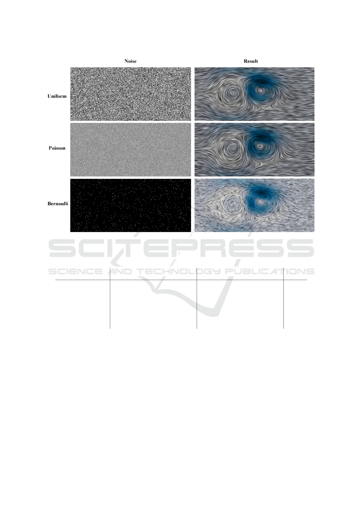
Figure 2: Noise distribution comparison. Our formulation is able to provide consistent results independently from the
random noise image considered. In the figure a comparison between uniform, Poisson and Bernoulli noise.
Table 2: Comparison between classical LIC with various interpolators/integrators, FLIC, and LIC-R (average processing time
in seconds).
LIC FLIC LIC-R
Dataset Lin./Euler Lin./RK4 Cub./Euler Lin./Euler Lin./RK4 Cub./Euler Order 4
jungtelziemniak2d 0.657 1.441 1.677 0.124 0.269 0.268 0.129
beads2d 0.105 0.239 0.284 0.012 0.017 0.017 0.052
boussinesq2d 0.606 1.405 1.319 0.138 0.154 0.173 0.150
cylinder2d 0.484 1.196 1.428 0.070 0.253 0.251 0.115
doublegyre2d 0.311 0.723 0.854 0.042 0.088 0.088 0.089
forcedampedduffing2d 0.105 0.241 0.294 0.011 0.016 0.016 0.025
fourcenters2d 0.116 0.369 0.284 0.012 0.020 0.020 0.043
pipedcylinder2d 0.504 1.029 1.222 0.168 0.202 0.200 0.104
between the C
1
and C
2
interpolators, we did not de-
rive a “septic” C
3
-continuous version that would be
the ideal pairing for the classical 4
th
order Runge-
Kutta scheme. For both classic LIC and Fast LIC,
we re-normalize vectors after interpolation to approx-
imate spherical interpolation and conserve arc-length
parameterization.
Fast LIC. Our implementation of the Fast LIC al-
gorithm leverages the same integrators and samplers
used for classic LIC, while exploiting streamline re-
dundancy that occurs in LIC as a new streamline is
always advected for each pixel despite the fact that
many pixels are hit by the same streamline (Stalling
and Hege, 1995). We consider equidistant streamline
sampling in combination with a box kernel to convert
texture convolution to a texture-averaging operation.
Thus, a streamline obtained to determine a pixel value
can be reused with only minor corrections (due to
the bi-directional kernel offset along the streamline)
since two immediate neighboring pixels have nearly
the same correlated pixels as their texture contribu-
tors. We maintain a pixel hit buffer to evaluate stream-
line coverage in the flow field, and therefore, only a
small number of streamlines are actually advected for
all pixels to collect texture contributions.
Noise Distributions. We tested our method on a va-
riety of sparse noise patterns, generated through the
Mersenne Twister random number generator (Mat-
LIC-R: Line Integral Convolution Revisited
881

Figure 3: Double gyre comparison. From left to right, our LIC-R formulation, classic LIC, and Fast LIC. From top to
bottom, for LIC-R: 2
nd
and 4
th
order derivative stencil; for Classic LIC and Fast LIC: linear and cubic with Runge-Kutta 4th
order integration. Note that Fast LIC has a crisper appearance due to the limited number of integration steps, while LIC-R
provides a smoother appearance.
sumoto and Nishimura, 1998) according to the fol-
lowing distributions:
• Uniform. We use the standard uniform genera-
tor that produces random floating-point values x,
uniformly distributed on the interval [a,b), that
is, distributed according to the probability density
function (Goualard, 2022):
P(x|a,b) =
1
b − a
.
• Poisson. We use the standard Poisson generator
that produces random non-negative integer val-
ues i, distributed according to discrete probability
function (Inouye et al., 2017):
P(i|µ) =
e
−µ
µ
i
i!
The value obtained is the probability of exactly
i occurrences of a random event if the expected,
mean number of its occurrence under the same
conditions (on the same time/space interval) is µ.
• Bernoulli. We use the standard Bernoulli genera-
tor that produces random boolean values, accord-
ing to the discrete probability function (Dai et al.,
2013). The probability of true is
P(b|p) =
(
p, if b is true
1 − p, if b is false
In Fig. 2 we show examples of our method ap-
plied to a vector field with different noise distribu-
tions. The results showcased in this manuscript are
generated with uniform noised distribution.
5 RESULTS
Figure 4: Boussinesq comparison: Left: LIC-R
th
order.
Center: Classic LIC with cubic interpolator and Runge-
Kutta 4
th
integrator. Right: Fast LIC with cubic interpolator
and Runge-Kutta 4
th
order integrator.
We benchmarked our method against the clas-
sical LIC (Cabral and Leedom, 1993) and the fast
LIC (Stalling and Hege, 1995) on a variety of
commonly-used 2D datasets: the simulation of a flow
around a cylinder (von-Karman Vortex Street, “cylin-
der”), a simulation of a viscous 2D flow around two
cylinders (“piped”), the simulation of a 2D flow gen-
erated by a heated cylinder in which the Boussinesq
approximation is used (“boussinesq2d”), an analyti-
cal periodic time-dependent vector field, in which a
IVAPP 2025 - 16th International Conference on Information Visualization Theory and Applications
882

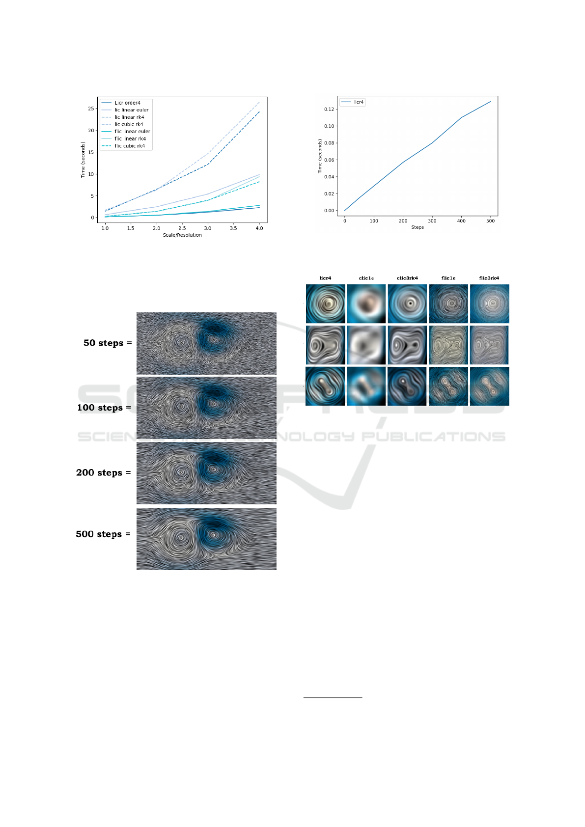
Figure 5: Execution time comparison: The plot shows the
performance of several numerical techniques, The x-axis
represents the resolution scale, while the y-axis reflects the
computation time in seconds. The result highlights LIC-R
4
th
order maintains execution times comparable to Fast LIC
across the scales.
Figure 6: LIC-R convergence: From top to bottom, the
LIC-R 4
th
order for a varying number of Gauss-Seidel steps.
separating boundary oscillates horizontally between
two oppositely rotating vortices (“double-gyre”), an
analytic data set of a rotating Petri dish, in which the
vortex center moves on a circular path (Weinkauf and
Theisel, 2010) (“petri”), an analytic data set contain-
ing four vortices (“four”), an analytic vector field de-
scribing the phase space of a duffing oscillator with
forcing and damping (“duffing”), a synthetic vector
field representing a von-Karman vortex street genera-
Figure 7: LIC-R complexity: The graph shows the compu-
tation time for LIC-R 4
th
order at the varying of integration
steps, showcasing the linear complexity.
Figure 8: Qualitative results: From left to right, compari-
son of our method (LIC-R order 4) with Classic LIC (linear
plus Euler, and cubic plus Runge-Kutta 4
th
order), and Fast
LIC (linear plus Euler, and cubic plus Runge-Kutta 4
th
or-
der). From top to bottom, beads2d, forceddampedduffing,
and fourcenters. Note that Fast LIC has a crisper appear-
ance due to the limited number of integration steps, while
LIC-R provides a smoother appearance.
tion and constructed as co-gradient to a stream func-
tion (“jungtel”). The datasets can be downloaded
from ETH Zurich’s repository
1
. The tests were per-
formed on a Razer Blade Stealth laptop equipped with
a CPU Intel i7-8565U, 4 cores at 1.8 GHz. For vi-
sualization purposes, we show the vector field mod-
ulus/magnitude color-mapped through ColorBrewer’s
colormap PuBu (Purple-Blue). For comparison, we
considered the classic and the Fast LIC formulation
with a variety of samplers and integrators: namely,
the samplers range from linear up to cubic order,
while the integrators range from the simple Euler up
to the 4
th
order Runge-Kutta. Table 2 shows the av-
erage processing times in seconds for our method
compared to various versions of LIC: our formula-
tion is three times faster than the simplest LIC im-
plementation (linear sampler with Euler integrator),
1
https://cgl.ethz.ch/research/visualization/data.php
LIC-R: Line Integral Convolution Revisited
883

and one order of magnitude faster than more complex
LIC formulations (cubic sampling through Catmull-
Rom splines and integration through 4
th
order Runge-
Kutta), while at the same time is maintaining com-
putation time comparable to Fast LIC implementa-
tion. Figure 5 compares LIC-R execution times for
the jungtelziemniak2d dataset with classic LIC and
fast LIC across different image scaling factors. It
showcases that computation times are comparable to
fast LIC, which involves a significant implementa-
tion overhead due to caching of partial characteristic
lines. Figure 7 shows the computation times for the
jungtelziemniak2d dataset obtained with different it-
eration steps, showcasing that our method has linear
complexity with respect to the number of steps. Fig-
ure 6 shows the output of LIC-R 4
th
order for differ-
ent integration steps. Our examples also corroborate
that higher order integrators need to be paired with
higher order interpolators, as shown in Fig. 3, Fig. 4
and Fig. 8, and as highlighted in (Stalling, 1998) the-
sis. In these figures, we provide qualitative compar-
isons between the classic LIC with different samplers
and integrators and our method. We use a 3-tap tent
filter and 500 × 1 pixel iterations for all classic LIC
figures in this paper, and 500 iterations with β = 0.2
for LIC-R, while we use a 51-tap triangular kernel for
Fast LIC and 5 iterations. We believe it is evident
that LIC-R provides a quality comparable to the orig-
inal method using Catmull-Rom interpolation and 4
th
order Runge-Kutta integration. In paticular, we ob-
serve that classic LIC tends to blur the resulting image
earlier, which we conjecture is a result of accumulat-
ing more numerical round-off errors, while fast LIC
provides crisper images but the coherent trajectories
seem to be shorter when compared to LIC-R. This
can arguably remedied by using bigger kernel sizes
but this choice comes at a computational penalty. The
accompanying video provides additional examples.
Limitations. We already highlighted the role of
stationary points but would argue that such points
are better added to the visualization using additional
methodology that is orthogonal to LIC. Another limi-
tation of our method is that, in the current implemen-
tation, we cannot control the convolution kernel κ,
the kernel arises naturally as the solution to the cur-
vature flow problem. A minor limitation is the non-
isometric version of the derivative stencils used in this
work: our stencils only have a 90
◦
rotational invari-
ance, yet previous work shows that using stencils with
higher rotational invariances (or even isometric sten-
cils) can result in substantially better results (Kamgar-
Parsi et al., 1999). In our method, the construction
of isometric differential stencils is hindered, but we
believe it is not made impossible by the use of direc-
tional derivatives.
6 CONCLUSIONS
We have presented a novel formulation of the orig-
inal LIC algorithm that takes inspiration of material
derivatives: material (the noise image) is smoothed
out along streamlines using curvature flow. Unlike
previous methods, we take a fully Eulerian view of
the problem, resulting in significant improvements in
terms of speed and ease-of-implementation over the
classical formulation.
In the future, we plan to improve the isometry
of our derivative stencils and investigate how cus-
tom smoothing kernels can be integrated into the
framework. We also plan to apply the method to
2-manifolds embedded in 3D space by combining
our method with approaches such as the Closest
Point Method (MacDonald and Ruuth, 2008; Auer
et al., 2012) for solving partial differential equa-
tions. A GPU-based implementation is likewise on
our agenda, as is a closer look at the material deriva-
tive formulation for unsteady flows. Note that our
method only has one pre-requisite, the formulation of
a directional, second-order derivative, which is well-
studied on 2-manifolds in the context of curvature.
However, sampling the noise image I in the vicin-
ity of the 2-manifold is non-trivial, and more research
with a special attention to computational demands is
needed.
REFERENCES
Agranovsky, A., Camp, D., Garth, C., Bethel, E. W.,
Joy, K. I., and Childs, H. (2014). Improved
post hoc flow analysis via lagrangian representa-
tions. In IEEE Symposium on Large Data Analy-
sis and Visualization (LDAV), pages 67–75. DOI:
10.1109/LDAV.2014.7013206.
Auer, S., MacDonald, C. B., Treib, M., Schneider, J.,
and R
¨
udiger, W. (2012). Real-time fluid effects
on surfaces using the closest point method. Com-
puter Graphics Forum, 31(6):1909–1923. DOI:
10.1111/j.1467-8659.2012.03071.x.
Bujack, R. and Middel, A. (2020). State of the art
in flow visualization in the environmental sciences.
Environmental Earth Sciences, 79(2):65. DOI:
10.1007/s12665-019-8800-4.
Bujack, R., Yan, L., Hotz, I., Garth, C., and Wang, B.
(2020). State of the art in time-dependent flow topol-
ogy: Interpreting physical meaningfulness through
mathematical properties. Computer Graphics Forum,
39(3):811–835. DOI: 10.1111/cgf.14037.
IVAPP 2025 - 16th International Conference on Information Visualization Theory and Applications
884

Cabral, B. and Leedom, L. C. (1993). Imaging vector fields
using line integral convolution. In ACM SIGGRAPH,
pages 263–270. DOI: 10.1145/166117.166151.
Calvetti, D., Morigi, S., Reichel, L., and Sgallari, F. (2000).
Tikhonov regularization and the l-curve for large dis-
crete ill-posed problems. Journal of Computational
and Applied Mathematics, 123(1):423–446. Numeri-
cal Analysis 2000. Vol. III: Linear Algebra.
Catmull, E. and Rom, R. (1974). A class of local interpo-
lating splines. In Computer Aided Geometric Design,
pages 317–326.
Chow, E., Anzt, H., Scott, J., and Dongarra, J. (2018). Us-
ing jacobi iterations and blocking for solving sparse
triangular systems in incomplete factorization precon-
ditioning. Journal of Parallel and Distributed Com-
puting, 119:219–230.
Dai, B., Ding, S., and Wahba, G. (2013). Multivariate
Bernoulli distribution. Bernoulli, 19(4):1465–1482.
Daßler, N. and G
¨
unther, T. (2024). Variational feature ex-
traction in scientific visualization. ACM Transactions
on Graphics (TOG), 43(4):1–16.
Delmarcelle, T. and Hesselink, L. (2023). A unified frame-
work for flow visualization. In Computer Visualiza-
tion, pages 129–170. CRC Press.
Farin, G. (2001). Curves and Surfaces for CAGD: A Prac-
tical Guide. Morgan Kaufmann, 5
th
edition. (Chapter
11).
Forsell, L. and Cohen, S. (1995). Using line integral
convolution for flow visualization: curvilinear grids,
variable-speed animation, and unsteady flows. IEEE
Transactions on Visualization and Computer Graph-
ics, 1(2):133–141. DOI: 10.1109/2945.468406.
Garth, C., Gerhardt, F., Tricoche, X., and Hans, H. (2007).
Efficient computation and visualization of coherent
structures in fluid flow applications. IEEE Trans-
actions on Visualization and Computer Graphics,
13(6):1464–1471. DOI: 10.1109/TVCG.2007.70551.
Goualard, F. (2022). Drawing random floating-point num-
bers from an interval. ACM Transactions on Modeling
and Computer Simulation (TOMACS), 32(3):1–24.
G
¨
unther, T. (2020). Visibility, topology, and inertia:
New methods in flow visualization. IEEE Computer
Graphics and Applications, 40(2):103–111. DOI:
10.1109/10.1109/MCG.2019.2959568.
G
¨
unther, T., Gross, M., and Theisel, H. (2017). Generic
objective vortices for flow visualization. ACM
Transactions on Graphics, 36(4):Art. #141. DOI:
10.1145/3072959.3073684.
G
¨
unther, T. and Theisel, H. (2018). The state of the
art in vortex extraction. Computer Graphics Forum,
37(6):149–173. DOI: 10.1111/cgf.13319.
G
¨
unther, T. and Theisel, H. (2024). Objective lagrangian
vortex cores and their visual representations. IEEE
Transactions on Visualization and Computer Graph-
ics.
Hadwiger, M., Mlejnek, M., Theußl, T., and Rautek, P.
(2019). Time-dependent flow seen through approx-
imate observer killing fields. IEEE Transactions on
Visualization and Computer Graphics, 25(1):1257–
1266. DOI: 10.1109/TVCG.2018.2864839.
Hanser, K., Meggendorfer, S., H
¨
ugel, P., Fallenb
¨
uchel,
F., Fahad, H. M., and Sadlo, F. (2019). Energy-
based visualization of 2d flow fields. In VISI-
GRAPP (3: IVAPP), pages 250–258. DOI:
10.5220/0007359602500258.
Hofmann, L. and Sadlo, F. (2021). Local extraction of 3d
time-dependent vector field topology. In Computer
Graphics Forum, volume 40, pages 111–122. Wiley
Online Library.
Inouye, D. I., Yang, E., Allen, G. I., and Ravikumar, P.
(2017). A review of multivariate distributions for
count data derived from the poisson distribution. Wi-
ley Interdisciplinary Reviews: Computational Statis-
tics, 9(3):e1398.
Interrante, V. (1997). Illustrating surface shape in vol-
ume data via principal direction-driven 3D line inte-
gral convolution. In ACM SIGGRAPH, pages 109—-
116. DOI: 10.1145/258734.258796.
Jakob, J., Gross, M., and G
¨
unther, T. (2021). A fluid flow
data set for machine learning and its application to
neural flow map interpolation. IEEE Transactions on
Visualization and Computer Graphics, 27(2):1279–
1289. DOI: 10.1109/TVCG.2020.3028947.
Jenny, B. (2021). Terrain generalization with line
integral convolution. Cartography and Geo-
graphic Information Science”, 48(1):78–92. DOI:
10.1080/15230406.2020.1833762.
Kamgar-Parsi, B., Kamgar-Parsi, B., and Rosenfeld, A.
(1999). Optimally isotropic laplacian operator. IEEE
Transactions on Image Processing, 8(10):1467–1472.
DOI: 10.1109/83.791975.
Kim, B. and G
¨
unther, T. (2019). Robust reference frame
extraction from unsteady 2D vector fields with convo-
lutional neural networks. Computer Graphics Forum,
38(3):285–295. DOI: 10.1111/cgf.13689.
Laramee, R. S., Erlebacher, G., Garth, C., Schafhitzel,
T., Theisel, H., Tricoche, X., Weinkauf, T., and
Weiskopf, D. (2008). Applications of texture-based
flow visualization. Engineering Applications of Com-
putational Fluid Mechanics, 2(3):264–274. DOI:
10.1080/19942060.2008.11015227.
Lawonn, K., Krone, M., Ertl, T., and Preim, B. (2014).
Line integral convolution for real-time illustration
of molecular surface shape and salient regions.
Computer Graphics Forum, 33(3):181–190. DOI:
10.1111/cgf.12374.
MacDonald, C. B. and Ruuth, S. J. (2008). Level
set equations on surfaces via the closest point
method. Scientific Computing, 35(2–3):219–240.
DOI: 10.1007/s10915-008-9196-6.
Matsumoto, M. and Nishimura, T. (1998). Mersenne
twister: a 623-dimensionally equidistributed uniform
pseudo-random number generator. ACM Transactions
on Modeling and Computer Simulation (TOMACS),
8(1):3–30.
McGraw, T., Vemuri, B. C., Wang, Z., Chen, Y., Rao, M.,
and Mareci, T. (2002). Line integral convolution for
visualization of fiber tract maps from DTI. In Med-
ical Image Computing and Computer-Assisted Inter-
vention (MICCAI), pages 615–622. DOI: 10.1007/3-
540-45787-9
77.
LIC-R: Line Integral Convolution Revisited
885

Rautek, P., Mlejnek, M., Beyer, J., Troidl, J., Pfister, H.,
Theußl, T., and Hadwiger, M. (2021). Objective
observer-relative flow visualization in curved spaces
for unsteady 2d geophysical flows. IEEE Transactions
on Visualization and Computer Graphics, 27(2):283–
293. DOI: 10.1109/TVCG.2020.3030454.
Rautek, P., Zhang, X., Woschizka, B., Theußl, T., and Had-
wiger, M. (2023). Vortex lens: Interactive vortex core
line extraction using observed line integral convolu-
tion. IEEE Transactions on Visualization and Com-
puter Graphics.
Rezk-Salama, C., Hastreiter, P., Teitzel, C., and Ertl, T.
(1999). Interactive exploration of volume line integral
convolution based on 3D-texture mapping. In IEEE
Visualization, pages 233–528. DOI: 10.1109/VI-
SUAL.1999.809892.
Rojo, I. B. and G
¨
unther, T. (2020). Vector field
topology of time-dependent flows in a steady ref-
erence frame. IEEE Transactions on Visualiza-
tion and Computer Graphics, 26(1):280–290. DOI:
10.1109/TVCG.2019.2934375.
Sadlo, F. and Peikert, R. (2007). Efficient visualization of
lagrangian coherent structures by filtered amr ridge
extraction. IEEE transactions on visualization and
computer graphics, 13(6):1456–1463.
Stalling, D. (1998). Fast Texture-Based Algorithms for Vec-
tor Field Visualization. PhD thesis, Konrad-Zuse Zen-
trum, Berlin. ZIB Opus4.
Stalling, D. and Hege, H.-C. (1995). Fast and
resolution independent line integral convolution.
In ACM SIGGRAPH, pages 249––256. DOI:
10.1145/218380.218448.
Sun, B. (2020). Correct expression of the material deriva-
tive in continuum physics. Preprints.
Sundquist, A. (2003). Dynamic line integral convolution for
visualizing streamline evolution. IEEE Transactions
on Visualization and Computer Graphics, 9(3):273–
282. DOI: 10.1109/TVCG.2003.1207436.
Telea, A. and van Wijk, J. J. (2003). 3D IBFV:
Hardware-accelerated 3D flow visualization. In IEEE
Visualization, pages 223–240. DOI: 10.1109/VI-
SUAL.2003.1250377.
van Wijk, J. J. (2003). Image based flow visualization for
curved surfaces. In IEEE Visualization, pages 123–
130. DOI: 10.1109/VISUAL.2003.1250363.
Wegenkittl, R., Groller, E., and Purgathofer, W. (1997). An-
imating flow fields: rendering of oriented line integral
convolution. In Computer Animation, pages 15–21.
DOI: 10.1109/CA.1997.601035.
Weinkauf, T. and Theisel, H. (2010). Streak lines as tangent
curves of a derived vector field. IEEE Transactions on
Visualization and Computer Graphics, 16(6):1225–
1234. DOI: 10.1109/TVCG.2010.198.
Yau, N. (2024). Visualize this: the FlowingData guide to
design, visualization, and statistics. John Wiley &
Sons.
Zhang, X., Hadwiger, M., Theußl, T., and Rautek, P. (2022).
Interactive exploration of physically-observable ob-
jective vortices in unsteady 2D flow. IEEE Trans-
actions on Visualization and Computer Graphics,
28(1):281–290. DOI: 10.1109/TVCG.2021.3115565.
IVAPP 2025 - 16th International Conference on Information Visualization Theory and Applications
886