Estimate Reference Evapotranspiration Using Machine Learning
Methods
Marwa Dorai
1,2 a
, Mehrez Abdellaoui
2 b
, Bouthaina Douh
3 c
and Ali Douik
2 d
1
University of Sousse, ISITCOM, 4011, Sousse, Tunisia
2
University of Sousse, ENISO, NOCCS Research Laboratory, 4054, Sousse, Tunisia
3
University of Sousse, ISA-CM, 4042 Sousse, Tunisia
Keywords:
Reference Evapotranspiration ET
0
, Machine Learning (ML), Internet of Things IoT, Water Stress.
Abstract:
Agriculture, a fundamental pillar of human civilisation, not only provides the food we need to survive, but
is also a major driver of global economic growth. Yet this critical sector is increasingly threatened by the
escalating impacts of climate change, particularly through the exacerbation of water scarcity in key agricul-
tural regions. Changing climate patterns are disrupting rainfall cycles, leading to more frequent droughts and
reduced water availability. As the global population grows exponentially and demand rises, farmers require
water for irrigation to meet these needs. This growing resource scarcity underscores the urgent need for inno-
vative, sustainable agricultural solutions to adapt to these challenges. To secure the future of water resources
and safeguard agricultural productivity, it is crucial to proactively implement cutting-edge technologies such
as the Internet of Things (IoT) and Artificial Intelligence (AI). In this context, we present a novel approach
for estimating reference evapotranspiration ET
0
with the aim of minimising water waste and improving the
efficiency of irrigation water management. The study was carried out in a real-world setting where several
sensors were installed to measure various parameters, including temperature, soil moisture and rainfall. The
station is connected to a server application from which a dataset was generated after data cleaning and pre-
processing. The parameters obtained from the dataset were classified in terms of their correlation with the
output value ET
0
. Regression was then performed using various machine learning (ML) tools to predict water
stress. The developed algorithms resulted in good performances in terms of coefficient of determination R
2
and loss function RMSE. These performances exceed those of existing methods from the state of the art.
1 INTRODUCTION
The water crisis has recently intensified into one of
the most urgent global challenges, particularly in the
Mediterranean region, where irrigation is vital for
maintaining and enhancing agricultural productivity.
The available water for agriculture in this region
is diminishing due to population growth and the in-
creasing frequency of droughts. This mounting pres-
sure on water resources necessitates the development
of strategies to enhance water use efficiency and opti-
mise the benefits derived from the available water.
one of the most effective strategies is the control
of the irrigation by considering the needs of the crops.
a
https://orcid.org/0000-0003-2442-3270
b
https://orcid.org/0000-0002-2492-5206
c
https://orcid.org/0000-0002-3439-2212
d
https://orcid.org/0000-0002-2492-5206
These needs can be estimated by measuring evap-
otranspiration (ET),is a key player in the water cy-
cle, moving water from soil and plants to sky through
evaporation and transpiration.
Understanding and estimating ET accurately is es-
sential for efficient water resource management and
irrigation planning. Crop water requirement is a fun-
damental aspect of irrigation water management. The
most effective way to define it is by reference evapo-
transpiration (ET
0
). ET
0
represents water evaporated
from the soil and emitted to the atmosphere by plants.
Accurate ET
0
calculations are essential for a wide
range of research, including irrigation planning, hy-
drological modeling, crop production forecasting and
sustainable water resource management at both local
and global scales. Additionally, ET information is
used as a basis for a number of international water
treaties and agreements, in particular with regard to
water allocation policies. Estimation of ET
0
from a
Dorai, M., Abdellaoui, M., Douh, B. and Douik, A.
Estimate Reference Evapotranspiration Using Machine Learning Methods.
DOI: 10.5220/0013131800003890
Paper published under CC license (CC BY-NC-ND 4.0)
In Proceedings of the 17th International Conference on Agents and Artificial Intelligence (ICAART 2025) - Volume 3, pages 343-350
ISBN: 978-989-758-737-5; ISSN: 2184-433X
Proceedings Copyright © 2025 by SCITEPRESS – Science and Technology Publications, Lda.
343

reference area can be achieved either by mathematical
modelling or by field trial data from specific sensors
such as lysimeters, followed by adjustment of the ET
0
value using empirical crop coefficients. While ET
0
can be precisely measured using field experiments
and lysimeters, this approach is often impractical due
to the high costs and significant time and energy re-
quired. Consequently, significant investment has been
made in research and development to create more effi-
cient mathematical models for estimating ET
0
. These
models typically utilise basic meteorological param-
eters, which are readily available locally. Significant
efforts are also being made to enhance the capabilities
of existing models and to develop new ones.There are
various indirect approaches to estimating ET
0
, rang-
ing from simple empirical models to more complex
ones. The choice of the most appropriate model de-
pends on several criteria, including data availability,
regional characteristics and the degree of precision re-
quired.
In recent years, there has been a notable shift in
the dominant methods for estimating ET
0
beginning
by advances in computer technology and the emer-
gence of numerical techniques such as ML and AI. In
(Bidabadi et al., 2024), the authors have demonstrated
that machine learning models, including neural net-
works and neuro-fuzzy systems, can outperform tra-
ditional methods such as the Penman-Monteith equa-
tion, especially in data-scarce environments. The
study demonstrated that ANFIS yielded the best re-
sults in estimating ET
0
using minimal input data, in-
cluding only temperature and wind speed from nearby
stations. In (Yassin et al., 2016), the authors assessed
the effectiveness of ANNs and gene expression pro-
gramming (GEP) in estimating ET
0
in arid climate.
The studies (Chia et al., 2020) and (Shrestha and
Shukla, 2015) have demonstrated that ANNs and sup-
port vector machines (SVM) are effective techniques
for determining and modelling actual crop ET using
climatic data. In (Adnan et al., 2017), the authors used
a range of machine learning techniques to develop a
model for estimating ET using reduced meteorologi-
cal parameters.
In this context, the use of artificial intelligence
techniques, particularly ML regression models, of-
fers significant potential for improving ET
0
estima-
tion. Unlike traditional approaches that often suffer
from the scarcity of meteorological data, ML models
can integrate a wide range of parameters, going be-
yond conventional meteorological data. These mod-
els can learn complex relationships between different
variables and provide accurate estimations even with
limited or incomplete data (Yong et al., 2023).
This research presents a ground-breaking multi-
parameter method for estimating ET
0
, integrating
state-of-the-art machine learning techniques and de-
tailed data analysis. This method aims to address the
shortcomings of conventional methods and provide
more reliable and accurate ET
0
estimates. Thereby,
we can contribute to create more efficient water re-
source management system and better irrigation plan-
ning in regions facing water scarcity.
The structure of this paper is as follows: follow-
ing the introduction, the second section covers the
approach and process, detailing the study site, the
weather station setup, data collection and process-
ing procedures, and the empirical approaches used.
The third section discusses the machine learning al-
gorithms employed. The fourth section focuses on the
evaluation metrics applied in the study. The fifth sec-
tion presents the results and discussion. Finally, the
paper concludes with a summary of the key findings
and offers suggestions for future research directions.
2 APPROACH AND PROCESS
2.1 Study Site
The study was performed at the Department of Horti-
cultural Systems and Natural Environments Engineer-
ing, Higher Agronomic Institute of Chott Mariem, lo-
cated in central-eastern Tunisia. The institute is lo-
cated at 35°91’ north latitude and 10°55’ east lon-
gitude, at an altitude of 19 metres above sea level.
This region belongs to the semi-arid bioclimatic zone,
characterised by mild winters and hot summers. A
meteorological station, situated 100 meters from the
experimental site, provided climatic data during the
study period. The average minimum and maxi-
mum temperatures were 14.94°C and 24.16°C, re-
spectively. Relative humidity averaged 69.14 % and
wind speed averaged 1.85 m/s. The average annual
rainfall in the area is 183.73 millimetres, with an
annual evaporation rate of 689.59 millimetres, with
a five-month drought period from May to Septem-
ber. The region is characterized by limited and in-
frequent precipitation, high evaporation rates, and el-
evated maximum temperatures.
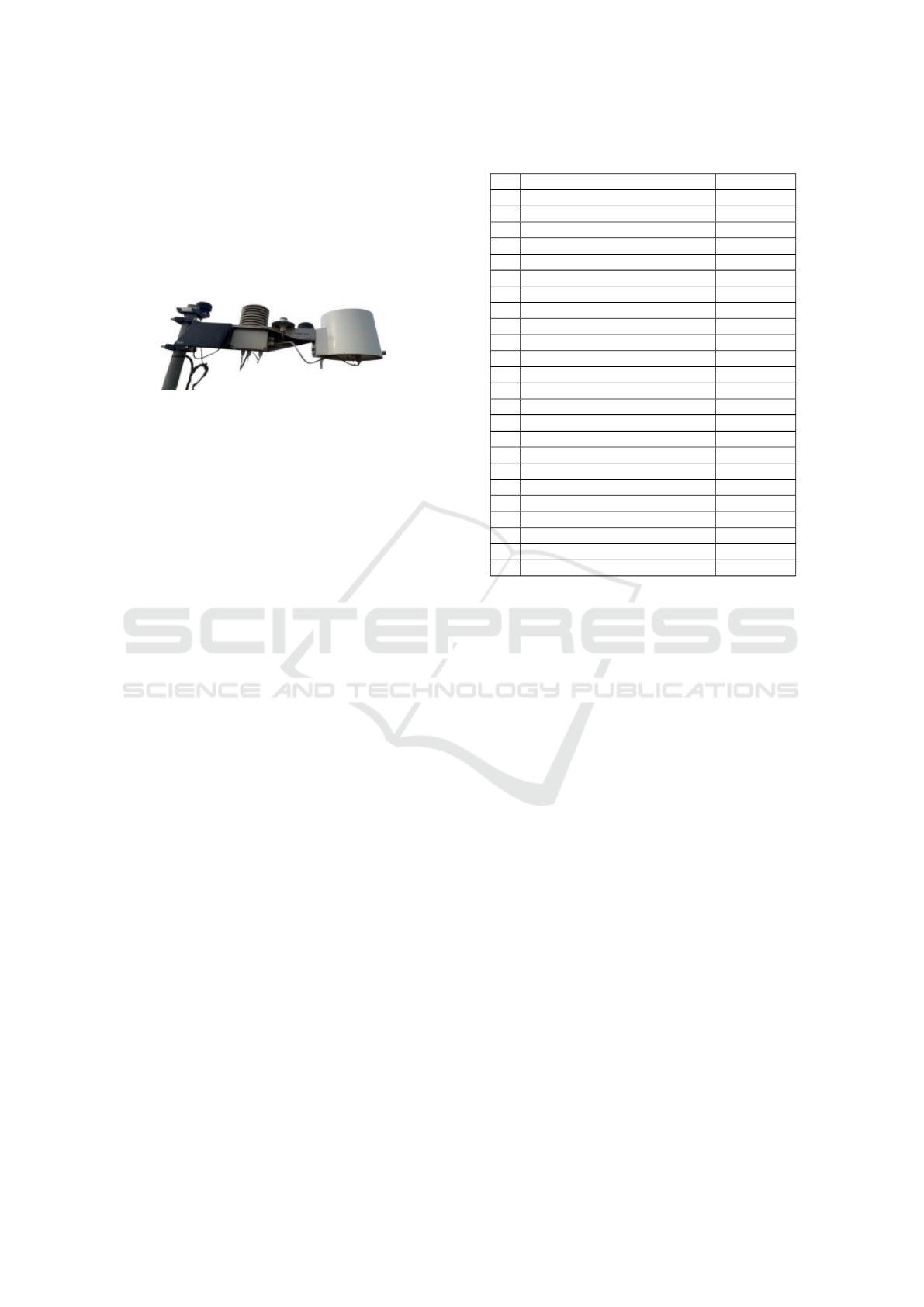
2.2 Weather Station Setup
The weather station is a comprehensive and au-
tonomous device designed to measure various cli-
matic parameters. It is equipped with several spe-
cific sensors that monitor temperature, humidity, wind
speed and direction, atmospheric pressure and precip-
itation levels. All these sensors are integrated into a
ICAART 2025 - 17th International Conference on Agents and Artificial Intelligence
344

central unit that collects data in real-time. To facili-
tate data transmission, the station is equipped with a
Wi-Fi module that sends the collected information to
the cloud every two hours. When data is required for
analysis, it is pre-processed to ensure its accuracy and
reliability. This pre-processing involves filtering out
anomalies and outliers that may result from sensor er-
rors or environmental disturbances.
Figure 1: Weather Station.
2.3 Data Collection and Processing
Procedures
The data collection and processing phase is critical to
ensuring the accuracy and usability of the climate data
collected by the weather station. This phase begins
with the transmission of data from the station to the
cloud via a Wi-Fi module. Every two hours, the accu-
mulated data is securely sent to a cloud-based storage
platform, Field Climate ensuring continuous and reli-
able data collection.
The Field Climate platform provides a compre-
hensive solution for managing and analyzing mete-
orological data collected by various weather stations.
It enables real-time monitoring of climatic conditions,
data storage, and analysis for applications such as pre-
cision agriculture or water stress detection.
The data is then preprocessed to improve its qual-
ity using various data-cleaning techniques. For exam-
ple, missing values, often caused by sensor failures
or transmission errors, are handled using imputation
methods such as mean, median, or last valid obser-
vation carried forward. This ensures that the dataset
remains complete and suitable for analysis.
In addition, data integrity is maintained by cor-
recting format errors and ensuring temporal con-
sistency, eliminating inconsistencies such as out-of-
sequence timestamps or duplicate entries. After
cleaning, the data is formatted and stored in CSV
(Comma-Separated Values) files. This standard for-
mat facilitates efficient data management and allows
for easy access and analysis. The structured storage
in CSV files includes feature values such as tempera-
ture, humidity, sunshine duration, and solar radiation,
as well as the target variable ET
0
, calculated using the
Penman formula. Table 1 illustrates all meteorologi-
cal parameters computed and saved in the dataset.
Table 1: List of the meteorological parameters.
Meteorological Parameters Abbreviations
1 Average soil moisture avg SM
2 Average soil temperature avg ST
3 Max soil temperature max ST
4 Min soil temperature min ST
5 Average air temperature avg AT
6 Max-Air-Temperature max-AT
7 Min-Air-Temperature min-AT
8 Dew Point DP
9 Min dew point min DP
10 Solar radiation SR
11 Vapor pressure deficit VDP
12 Min Vapor pressure deficit min VDP
13 HC-Relative-humidity HC-RH
14 Max-Relative-Humidity Max-RH
15 Min-Relative-Humidity Min-RH
16 Precipitation P
17 U-sonic wind speed U sws
18 Max wind speed Max ws
19 Wind gust w g
20 Delta D
21 Max delta Max D
22 Min delta Min D
23 Sunshine duration SD
24 Reference evapotranspiration ET
0
2.3.1 Empirical Methods
A number of empirical methods have been devel-
oped for the estimation of reference evapotranspira-
tion ET
0
. These methods employ a variety of climatic
data and empirical relationships in order to provide re-
liable estimates. The most widely recognised of these
methods are as follows:
2.3.2 Hargreaves-Samani Method (HS)
The HS method, developed by Hargreaves and
Samani, employs temperature data and extraterrestrial
radiation to estimate ET
0
. This method’s simplicity is
one of its main advantages, especially in areas with
scarce climatic data (Althoff et al., 2019).
2.3.3 Thornthwaite Method
This method created by C.W. Thornthwaite, it is a
popular choice due to its straightforward implemen-
tation and minimal data requirements. However, this
method is more applicable to humid regions and may
require adjustments for arid climates (Thornthwaite,
1948).
2.3.4 Blaney-Criddle Method (BC)
The Blaney-Criddle (BC) method, developed by H. F.
Blaney and W. D. Criddle, is a widely used approach
in agricultural water management for estimating crop
Estimate Reference Evapotranspiration Using Machine Learning Methods
345

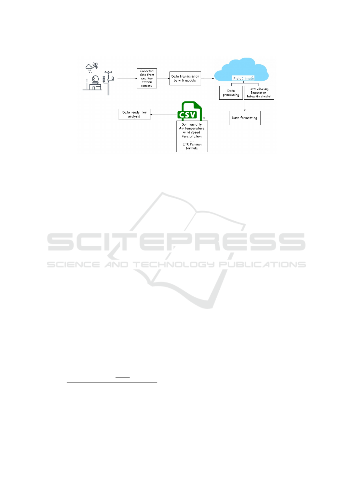
Figure 2: Data collection and processing workflow.
water requirements. It uses mean monthly tempera-
ture and the percentage of annual daylight hours. The
BC method has undergone several refinements to im-
prove its accuracy under different climatic conditions
(Sobrinho et al., 2020).
2.3.5 Priestley-Taylor Method (PT)
This methodology, developed by Priestley and Tay-
lor, modifies the Penman equation to estimate ET
0
in environments where radiation is the primary fac-
tor influencing evapotranspiration. This offers a more
efficient alternative to the original Penman equation,
with the introduction of an empirical coefficient, and
is particularly useful for humid regions with ample
solar radiation (Sobrinho et al., 2020)
2.3.6 Penman–Monteith Method (PM)
Howard Penman developed the Penman Method,
which integrates energy balance and aerodynamic
principles to calculate ET
0
. This method requires
detailed meteorological data, making it data inten-
sive but exceptionally accurate. The PM has been
standardised by the FAO and WMO (Sobrinho et al.,
2020), (Wright, 1985). Despite its complexity, the
Penman method is celebrated for its precision and is
widely accepted as the gold standard for ET
0
estima-
tion. As a result, the standardised ET
0
equation (1) is
used as the target variable in the modelling phases.
ET
0
=
0.408∆(R
c
− H) + ρ
900
T
a
+273
V
2
(P
s
− P
a
)
∆ + ρ(1 +0.34V
2
)
(1)
Defining the variables as follows:
• ET
0
: Reference ET (mm/day).
• R
c
: Crop surface net radiation (MJ/m
2
/day).
• H: Soil heat flux density (MJ/m
2
/day).
• T
a
: Average daily air temperature at 2 meters
above ground level(
◦
C).
• V
2
: Two-meter wind speed (m/s).
• P
s
: Saturation pressure of the water vapor (kPa).
• P
a
: Actual vapor pressure (kPa).
• P
s
− P
a
: Water vapor deficit (kPa).
• ∆: Temperature coefficient of saturation vapor
pressure (kPa/
◦
C).
• ρ: Moisture content coefficient (kPa/
◦
C).
3 MACHINE LEARNING
MODELS
This research explores the application of machine
learning models, including linear regression, random
forest, support vector regression and extreme gradient
boosting, to predict ET
0
. These methods are imple-
mented using Python, ensuring robust and consistent
results for this research endeavor.
3.1 Linear Regression
Linear Regression is a key method for modeling the
relationship between a target variable and one or more
predictor variables. The objective is to identify a
linear equation that best fits this relationship. This
is achieved by representing the target variable as a
weighted sum of the predictor variables, together with
an intercept. The coefficients are calculated by min-
imising a loss function, typically the sum of squared
errors. By assuming a linear relationship, Linear Re-
gression simplifies the modeling process, making it
effective for understanding and predicting patterns in
data, especially when the relationship is straightfor-
ward.
ICAART 2025 - 17th International Conference on Agents and Artificial Intelligence
346

3.2 Random Forest
RF implemented by (Breiman, 2001), is an ensem-
ble learning approach that consists of several decision
tree estimators. Each tree in the forest is constructed
from values derived from a randomly sampled subset
of the data. The process starts at the root node of each
tree and progresses downwards, evaluating all avail-
able information at each node. Predictive variables
are calculated throughout this process. To prevent
over-fitting, a cross-validation technique is employed,
which systematically trims the trees to enhance their
generalisability.
3.3 Spport Vector Regressor
SVR is a machine learning approach that integrates
the principles of Support Vector Machine (SVM) and
is utilized for non-linear regression (Vapnik, 2013).
The objective is to identify a function that accurately
approximates the relationship between input variables
and target values, while simultaneously minimising
both error and model complexity. The process begins
with fitting a linear model to the data, followed by
applying a nonlinear kernel to capture more intricate
patterns. The method focuses on minimising opera-
tional risk rather than just prediction error, making it
an effective approach for modelling intricate data re-
lationships.
3.4 Extreme Gradient Boosting
Algorithm (XGBoost)
XGBoost, developed by (Chen and Guestrin, 2016), is
a ML tool that a machine learning framework lever-
aging ensemble decision tree gradient boosting for
high predictive accuracy. It uses shrinkage (learn-
ing rate adjustment) to fine-tune predictions and re-
duce overfitting. Column subsampling enhances ro-
bustness by selecting random feature subsets, reduc-
ing correlation. Tree pruning, guided by a gamma
threshold, simplifies trees by removing insignificant
splits, while L1 and L2 regularization penalties pre-
vent model overcomplexity. XGBoost also handles
missing values natively, learns optimal paths without
imputation, and employs early stopping to avoid over-
fitting and save computational effort. These features
make it efficient and effective for diverse ML tasks.
4 EVALUATION PERFORMANCE
METRICS
The accuracy and performance of the ML models
in estimating ET
0
were evaluated using two widely
adopted regression metrics: the determination coeffi-
cient R
2
and the root-mean-square error (RMSE). The
R
2
is employed to asses the correlation and agreement
between the actual and predicted daily ET
0
values.
The value of R
2
varies between 0 and 1, with R
2
=
1 indicating a positive correlation. Whereas RMSE
is used to measure the error associated with the esti-
mated models. This metric ranges from 0 to infinity,
with lower RMSE values indicating that the model’s
predictions closely align with the actual values (Zhou
et al., 2020) (Zhou et al., 2020). The evaluation met-
rics are calculated using the following equations.
R
2
= 1 −
∑
N
i=1
(y
ri
− y
pi
)
2
∑
N
i=1
(y
ri
− ¯y
ri
)
2
(2)
RMSE =
s
1
N
N
∑
i=1
(y
ri
− y
pi
)
2
(3)
where :
• N: Total number of samples.
• y
r
i
: Real value of the i-th sample.
• y
p
i
: Predicted value of the i-th sample.
• ¯y
r
: Mean of the real values
5 RESULTS AND DISCUSSIONS
This study uses a dataset covering the period from
September 2022 to May 2024, which originally con-
tained 9946 rows by 61 columns (parameters). Af-
ter pre-processing, it was reduced to 610 rows and
24 variables. The dataset was then divided into two
subsets: 80% for training and 20% for testing. To
ensure reliable variable selection for reference evapo-
transpiration (ET
0
) estimation and to avoid data leak-
age, correlation coefficients were computed only from
the training set.
A correlation matrix is a tool for displaying corre-
lations among several variables. The correlations be-
tween two variables is represented in each cell of the
matrix. The coefficients vary between -1 and 1 and in-
dicated the magnitude and direction of their linear re-
lationship. A perfect correlation can only be detected
by a value of 1 or -1, while a value of 0 indicates that
none exists. (Agrawal et al., 2022). In this study, a
correlation matrix was employed to examine the rela-
tionships between various meteorological parameters
Estimate Reference Evapotranspiration Using Machine Learning Methods
347

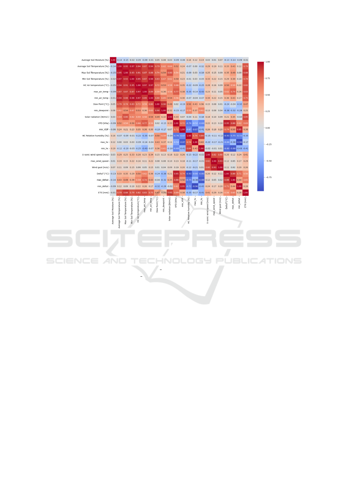
Figure 3: Inter-correlation Heatmap of Various Input Meteorological Parameters.
(inputs) and ET
0
as the output. The correlation coef-
ficients were computed exclusively from the training
data to ensure precise variable selection. The results,
illustrated in Figure 3 as a heatmap, show that Max
ST
has the greatest impact on ET
0
, while Avg SM has the
least significant effect.
Several tests and evaluations have been conducted
to achieve the best performance of the proposed
method. The idea of the test algorithm is to vary
the number of parameters used in the prediction algo-
rithm, considering their ranking from the top 3 to all
parameters. The evaluation of the regression scores
R
2
when varying the number of parameters involved
in the algorithm is shown in the figure below.
After analysing the results obtained, we can con-
clude that the number of parameters used for regres-
sion is crutial to reach the best performances. If we
choose 8 parameters or less, R
2
score doesn’t ex-
ceed 0.94. While, this score reaches the best values
when the number of parameters exceeds 13. Each
regression method has a unique sensitivity to differ-
ent sets of input parameters, which affects its per-
formance and accuracy. For example, some methods
may achieve optimal results with a larger set of pa-
rameters, such as LR with 22 parameters capturing
more complex patterns within the data. While oth-
ers, such as XGBoost with only 14 parameters, may
perform better with a more streamlined selection, re-
ducing the potential for overfitting and focusing on
the most influential variables. In addition to R
2
score,
we have computed RMSE for each combination of the
input parameters from the top 3 to all parameters. We
can conclude that when R
2
increases the RMSE de-
creases. Figure 5 illustrates the evolution of RMSE
values when varying the number of parameters. This
variability highlights the importance of tailoring the
parameter selection process to the specific character-
istics and requirements of each regression method. It
also highlights the need for a thorough evaluation and
comparison of different models to determine the most
effective approach for a given dataset and prediction
task. Ultimately, the choice of parameters and regres-
sion method is crucial in determining the precision
and reliability of the predictive model. To make the
right choice, table 2 summarises the best scores ob-
tained for each method and the number of parameters
involved. The data in this table allows us to gain valu-
able insights into the performance and complexity of
the four regression models. The SVR model achieves
the best R
2
value of 0.9764, with the LR and XG-
Boost models not far behind, both achieving a value
of 0.9759. The maximum R
2
for RF is 0.9622, which
ICAART 2025 - 17th International Conference on Agents and Artificial Intelligence
348

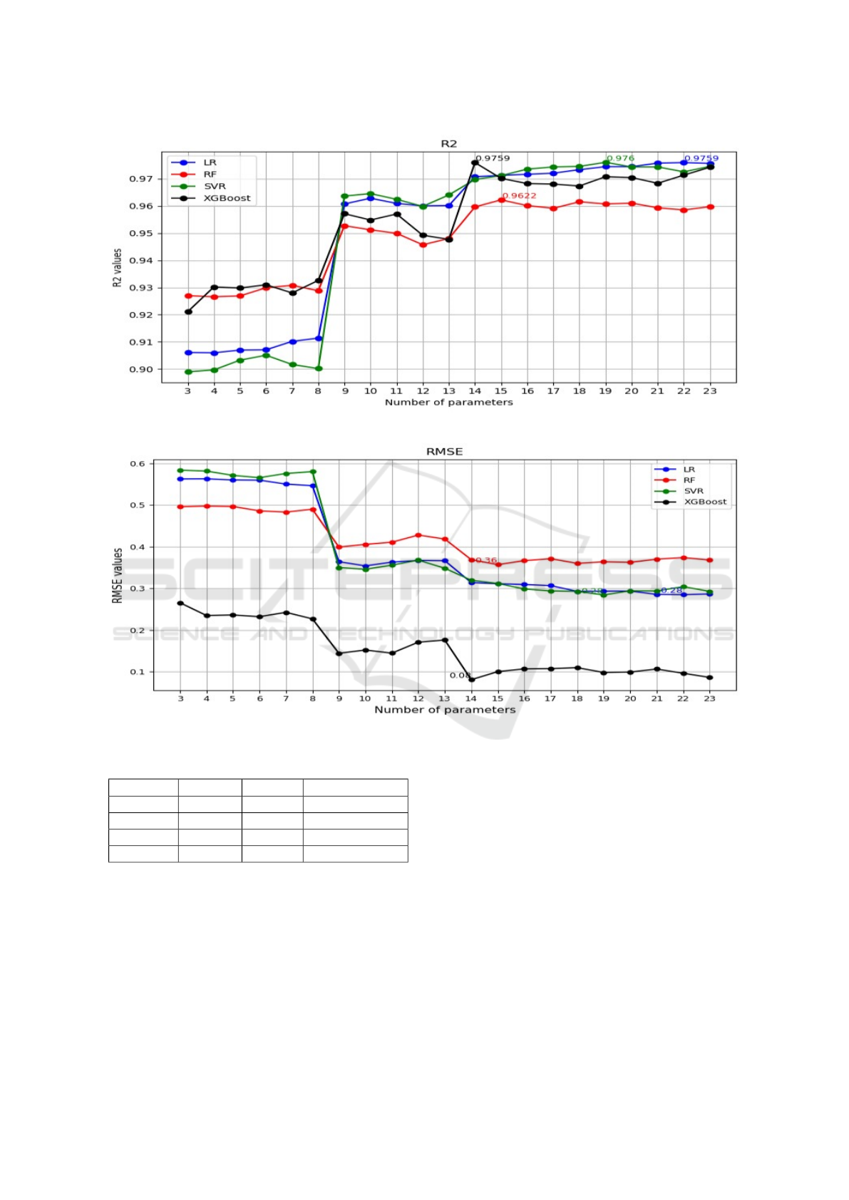
Figure 4: Evolution of R
2
score when varying the number of parameters.
Figure 5: Evolution of RMSE score when varying the number of parameters.
Table 2: Best results of evaluation metrics.
Models Max R
2
Min R
2
Param’s numb
LR 0.9759 0.2849 22
RF 0.9622 0.3568 15
SVR 0.9764 0.2814 19
XGBoost 0.9759 0.0811 14
is still a commendable result. In terms of RMSE,
XGBoost has the lowest value of 0.0811, indicating
superior prediction accuracy. The next lowest val-
ues were achieved by SVR and LR, with scores of
0.2814 and 0.2849, respectively. The highest RMSE
was recorded for RF, at 0.3568. In terms of the num-
ber of parameters, XGBoost uses the fewest number
equal to 14, which demonstrates that it is both high-
performing and relatively simple. Additionally, RF is
a relatively simple model with 15 parameters, while
SVR and LR are more complex, with 19 and 22 pa-
rameters, respectively. Overall, XGBoost is the most
effective model due to its lowest RMSE and minimal
number of parameters, making it the optimal choice
for precise predictions with reduced complexity. SVR
shows excellent Max R
2
,but is slightly less effective
in terms of RMSE. LR and RF are competitive, but do
not outperform the other models on key metrics.
6 CONCLUSIONS
This research sought to assess the effectiveness of var-
ious machine learning models in estimating ET
0
using
the FAO Penman method. The models tested included
Estimate Reference Evapotranspiration Using Machine Learning Methods
349

linear regression, random forest, support vector re-
gression, and XGBoost. These tests were conducted
by varying the number of meteorological parameters,
ranging from the three most correlated to ET
0
to the
complete set of parameters. Our findings demonstrate
that the efficacity of the models is clearly influenced
by the algorithm employed and the number of param-
eters incorporated into the predictions. In general,
more sophisticated algorithms such as SVR and XG-
Boost demonstrated superior performances, although
each model exhibited particular strengths depending
on the evaluation metrics used. In conclusion, the
study emphasises the significance of algorithm selec-
tion and parameter inclusion for enhancing the preci-
sion of ET
0
estimations. The XGBoost model demon-
strated particular effectiveness in terms of RMSE, in-
dicating its capacity to provide highly accurate esti-
mations with relatively few parameters. The choice
of algorithm for ET
0
estimation is significantly influ-
enced by the available parameters and data. For appli-
cations requiring high precision, models like SVR and
XGBoost are recommended. However, future studies
could focus on hyperparameter optimisation and the
use of ensemble techniques to potentially further en-
hance estimation performance.
ACKNOWLEDGEMENTS
We are extremely grateful to the Department of Hor-
ticultural Systems and Natural Environments Engi-
neering at the Higher Agronomic Institute of Chott
Mariem for their generous support. It is a true honor
to have been entrusted with access to your confiden-
tial information, and we deeply appreciate your trust
in our work.
REFERENCES
Adnan, M., Latif, M. A., Nazir, M., et al. (2017). Estimat-
ing evapotranspiration using machine learning tech-
niques. International journal of advanced computer
science and applications, 8(9):108–113.
Agrawal, Y., Kumar, M., Ananthakrishnan, S., and Kumara-
puram, G. (2022). Evapotranspiration modeling using
different tree based ensembled machine learning al-
gorithm. Water Resources Management, 36(3):1025–
1042.
Althoff, D., Santos, R. A. d., Bazame, H. C., Cunha, F.
F. d., and Filgueiras, R. (2019). Improvement of
hargreaves–samani reference evapotranspiration esti-
mates with local calibration. Water, 11(11):2272.
Bidabadi, M., Babazadeh, H., Shiri, J., and Saremi, A.
(2024). Estimation reference crop evapotranspira-
tion (et0) using artificial intelligence model in an arid
climate with external data. Applied Water Science,
14(1):3.
Breiman, L. (2001). Random forests. Machine learning,
45:5–32.
Chen, T. and Guestrin, C. (2016). Xgboost: A scalable
tree boosting system. In Proceedings of the 22nd acm
sigkdd international conference on knowledge discov-
ery and data mining, pages 785–794.
Chia, M. Y., Huang, Y. F., and Koo, C. H. (2020). Support
vector machine enhanced empirical reference evapo-
transpiration estimation with limited meteorological
parameters. Computers and Electronics in Agricul-
ture, 175:105577.
Shrestha, N. and Shukla, S. (2015). Support vector machine
based modeling of evapotranspiration using hydro-
climatic variables in a sub-tropical environment. Agri-
cultural and forest meteorology, 200:172–184.
Sobrinho, O. P. L., J
´
unior, W. L. C., dos Santos, L. N. S.,
da Silva, G. S., Pereira,
´
A. I. S., and Tavares, G. G.
(2020). Empirical methods for reference evapotran-
spiration estimation. Scientia Agraria Paranaensis,
pages 203–210.
Thornthwaite, C. W. (1948). An approach toward a ratio-
nal classification of climate. Geographical review,
38(1):55–94.
Vapnik, V. (2013). The nature of statistical learning theory.
Springer science & business media.
Wright, J. L. (1985). Evapotranspiration and irrigation wa-
ter requirements.
Yassin, M. A., Alazba, A., and Mattar, M. A. (2016). Ar-
tificial neural networks versus gene expression pro-
gramming for estimating reference evapotranspiration
in arid climate. Agricultural Water Management,
163:110–124.
Yong, S. L. S., Ng, J. L., Huang, Y. F., and Ang, C. K.
(2023). Estimation of reference crop evapotranspi-
ration with three different machine learning mod-
els and limited meteorological variables. Agronomy,
13(4):1048.
Zhou, Z., Zhao, L., Lin, A., Qin, W., Lu, Y., Li, J., Zhong,
Y., and He, L. (2020). Exploring the potential of deep
factorization machine and various gradient boosting
models in modeling daily reference evapotranspira-
tion in china. Arabian Journal of Geosciences, 13:1–
20.
ICAART 2025 - 17th International Conference on Agents and Artificial Intelligence
350