A Subspace Projection Based Technique for Visualizing Machine

Learning Models

Ziqian Bi

, Raymond Gao

and Shiaofen Fang

Purdue Polytechnic Institute, Purdue University, U.S.A.

Acton-Boxborough Regional High School, Acton, Massachusetts, U.S.A.

Department of Computer Science, Luddy School of Informatics, Computing and Engineering,

Indiana University Indianapolis, U.S.A.

Keywords: Machine Learning, Multi-Dimensional Data Visualization, Classification, Projection.

Abstract: As Artificial Intelligence (AI) technology, particularly Machine Learning (ML) algorithms, becomes

increasingly ubiquitous, our abilities to understand and interpret AI and ML algorithms become increasingly

desirable. Visualization is a common tool to help users understand individual ML decision-making processes,

but its use in demonstrating the global patterns and trends of a ML model has not been sufficiently explored.

In this paper, we present a visualization technique using subspace projection to visualize ML models as scalar

valued multi-dimensional functions to help users understand the global behaviors of the models in different

2D viewing spaces. A formal definition of the visualization problem will be given. The visualization technique

is developed using an interpolation-based subspace morphing algorithm and a subspace sampling method to

generate various renderings through projections and cross-sections of the model space as 3D surfaces or

heatmap images. Compared to existing ML visualization methods, our work provides better global views and

allows the users to select viewing spaces to provide user-specified perspectives. This method will be applied

to two real-world datasets and applications: the diagnosis of Alzheimer's Disease (AD) using a human brain

networks dataset and a real-world benchmark dataset for predicting home credit default risks.

1 INTRODUCTION

Machine learning (ML) algorithms act mostly as a

black box, i.e. the users have very little information

about how and why the algorithms work or fail. The

underlying ML models are also designed primarily

for the convenience of learning from data, but they

are not easy for the users to understand or interact

with. Explainable AI, particularly explainable ML

algorithms, is a critical area to ensure safety and trust

in the use of AI technologies in human society (Adadi

& Berrada, 2018). One of the most powerful tools in

developing explainable ML algorithms is

visualization (Chatzimparmpas, et al., 2020). Being

able to view the progression of a decision-making

process in a ML algorithm is often a desirable feature

for many critical AI applications (Seifert, et al.,

2017). While visualizing a local decision-making

process of an algorithm can provide useful insight

about the ML model, it would be beneficial if

visualization can be used to show the overall shape

pattern of the ML model itself in some space that the

users can understand. This type of global model

visualization has not been sufficiently studied,

primarily because it is very challenging to visualize a

high-dimensional function (as is the case with most

ML models) in a limited screen space.

Although high-dimensional data visualization

techniques (Liu, et al., 2017) can be applied to a set

of sample points computed by the model in the high-

dimensional space, the fact the model represents a

continuous function with intrinsic shape information

cannot be captured using traditional information

visualization techniques for discrete data set. Some

types of rendering methods are necessary to represent

the continuous shape patterns.

In this work, we focus on ML models that can be

defined as a scalar valued function in a high-

dimensional feature space, i.e. supervised single

valued model trained using a training dataset. The

training samples can also play an important role in the

visualization process. To this end, we can use volume

visualization as an analog when considering this

visualization problem (Kaufman, 1992). A typical

Bi, Z., Gao, R. and Fang, S.

A Subspace Projection Based Technique for Visualizing Machine Learning Models.

DOI: 10.5220/0013132100003912

Paper published under CC license (CC BY-NC-ND 4.0)

In Proceedings of the 20th International Joint Conference on Computer Vision, Imaging and Computer Graphics Theory and Applications (VISIGRAPP 2025) - Volume 1: GRAPP, HUCAPP

and IVAPP, pages 887-894

ISBN: 978-989-758-728-3; ISSN: 2184-4321

887

volume data such as a CT or MRI volume is a single

valued function defined over a 3D domain. If we

extend the 3D domain to an N-dimensional feature

space, it defines a ML model where the function

value is the learning label such as the classification

probability or value of a predictive regression model.

The rendering of such a model is, however, more

challenging for several reasons. First, the concepts of

depth cue and visual perception do not exist in high-

dimensional space. Therefore, traditional rendering

operations such as blending and shading do not apply.

Secondly, sampling in a higher dimensional

orthogonal subspace (for each pixel) to the viewing

space does not have a simple order. Thus, cross-

sections and projections will need to be carefully re-

defined to generate meaningful visual

representations. Third, when the dimensionality of

the feature space is high, a 2D screen space is a very

narrow and limited viewing window. Thus, the

selection of and interaction with the viewing spaces

are important for the understanding and interpretation

of the model.

In this paper, we propose a new visualization

technique to simulate a 3D volume rendering problem

for ML models. Our visualization technique uses an

interpolation-based subspace morphing algorithm

and a subspace sampling method to generate various

renderings through projections and cross-sections of

the model space as 3D surfaces or heatmap images.

We will also apply our visualization technique to two

real-world datasets and applications: the diagnosis of

Alzheimer's Disease (AD) using a human brain

networks dataset and a real-world benchmark dataset

for predicting home credit default risks

2 RELATED WORK

Applying visualization and visual analytics principles

in interactive or human-in-the-loop ML has become

an active research area in recent years

(Chatzimparmpas, et al., 2020). Most of the existing

studies focus on using visualization for understanding

local decision-making processes of ML models

(Seifert, et al., 2017). There are also some recent

works on using visual analytics to improve the

performance of ML algorithms through better feature

selection or parameter setting (Endert. et al., 2017;

May, et al., 2011).

Previous works on using visualization to help

understand the ML processes are usually designed for

specific types of algorithms, such as support vector

machines, neural networks, and deep learning neural

networks. Multi-dimensional visualization

techniques such as scatterplot matrix have been used

to depict the relationships between different

components of the neural networks (Zahavy, et al.,

2016; Rauber, et al., 2017). Typically, a learned

component is represented as a higher dimensional

point. The 2D projections of these points in either

principal component analysis (PCA) spaces or a

multi-dimensional scaling (MDS) space can better

reveal the relationships of these components that are

not easily understood, such as clusters and outliers.

Several methods apply graph visualization

techniques to visualize the topological structures of

the neural networks (Tzeng & Ma, 2005; Harley,

2015; Streeter, et al., 2001). Visual attributes of the

graph can be used to represent various properties of

the neural network models and processes.

Several recent studies addressed the challenges

of visualizing deep neural networks. In (Liu, et al.,

2017), a visualization system, CNNVis, was

developed to help ML experts understand deep

convolutional neural networks by clustering the

layers and neurons. Techniques have also been

developed to visualize the response of a deep neural

network to a specific input in a real-time dynamic

fashion (Yosinski, et al., 2015; Luisa, et al., 2017).

Observing the live activations that change in response

to user input helps build valuable intuitions about

how convnets work. There are several literatures that

discuss visualization’s roles in Support Vector

Machines. In (Lim, 2014), visualization methods

were used to provide access to the distance measure

of each data point to the optimal hyperplane as well

as the distribution of distance values in the feature

space. In (Hamel, 2006), multi-dimensional scaling

technique was used to project high-dimensional data

points and their clusters onto a two-dimensional map

maintaining the topologies of the original clusters as

much as possible to preserve their support vector

models. In (Wang, et al., 2016), interactive volume

visualization was used to identify potential features

for classification of brain network data. Finally,

Visualization were also used to analyze the

performances of ML algorithms in different

applications (Ren, et al., Alsallakh, et al., 2014; 2017;

Chuang, et al., 2013).

Compared to the visualization of local ML

processes, there have been relatively few known

techniques for the global visualization of a ML model

as a whole. The Manifold system (Zhang, et al., 2019)

provides a generic framework that does not rely on or

access the internal logic of the model and solely

observes the input and output. It applies scatter plot

matrix visualization to observe input and output

samples to evaluate model performance and behavior.

IVAPP 2025 - 16th International Conference on Information Visualization Theory and Applications

888

In (li, et al., 2018), scatter plots were used to visualize

ML models to help select the optimal set of training

samples.

Using subspace concepts to visualize high-

dimensional datasets has been explored in

information visualization. 2D linear projections from

unique linear subspaces are used to visualize high-

dimensional data in (Liu, et al., 2015). Singular value

decomposition is applied to the high dimensional data

to detect 1D subspaces for effective search and

exploration of generative models (Chiu, et al., 2020).

In (Gerber, et al., 2010), topological and geometric

techniques are used to approximate the high

dimensional data by Morse-Smale complex on the

cloud of point samples through parametric space

segmentation. A simplified geometric representation

of the Morse-Smale complex is then visualized by 2D

embedding. These techniques are designed for the

projection of discrete point data rather than a

continuous model or manifold where discrete points

cannot capture the true and continuous shape

information. Geometric and topological

approximation is also problematic as details of the

model, even if not smooth (e.g. rough boundaries),

are important information for interactive ML

3 PROBLEM DEFINITION

We only focus on, in this paper, the ML models that

can be defined as a scalar valued function in a high-

dimensional feature space, i.e. supervised single

valued model trained using a training dataset. This

type of ML model can be defined as a function:

𝐹(x





,…,x



)∶ 𝑅



→R

where 𝑅



is the n-dimensional feature space, and the

output is the result of the ML algorithm which can be

either a classification probability or a predicted

regression function value. We also assume that the

ML model is trained using a training set:

P={P





,…,P



}⊂R



and {F(P



):𝑖=

1⋯𝑛}⊂R

The visualization problem is hereby defined as an

image on a 2D viewing space

(

𝑢,𝑣

)

, representing

some information about the function F, projected

onto this 2D viewing space. The viewing space is

generally a 2D subspace of the feature space. The

meaning of projection here has two components:

1) Subspace determination: For each pixel in the

viewing space, find the subspace in the feature

space that are orthogonal to the viewing space at

this pixel point.

2) Subspace sampling: Within the orthogonal

subspace, determine what values should be used

to render this pixel. This is the process of

sampling or information filtering and integration

for visual presentation.

The visualization problem is now a problem of

projecting the n-dimensional function onto selected

2D viewing spaces. The high dimensionality makes

this projection less defined and under constrained.

Figure 1 shows a summary of this framework for a

viewing space (u,v) and an ML model F

Figure 1: An illustration of the visualization approach, F is

the ML model; (u,v) is the viewing space; 𝑃



are the training

set samples. Their projections on (u,v) space are 𝑃





; 𝐹



the subspace orthogonal to the pixel Q. This subspace will

be projected onto Q after information filtering and

sampling.

4 VISUALIZATION APPROACH

4.1 Viewing Space Selection

Viewing space,

(

𝑢,𝑣

)

, is a 2D subspace of the feature

space which the ML function will be projected onto.

The user will select two variables to represent the 2D

axes of the viewing space. Based on the following

criteria:

1) Interpretable variables. These are usually the

features that the users are familiar with, thus, can

be used to better understand the behavior of the

ML model.

2) Representative variables. These are the features

or variables (can be combinations of features)

that can capture the most amount of information

or variations of the ML model, such as the PCA

space.

In this work, we only consider viewing spaces that

are 2D linear subspaces of the feature space. An

important reason is interpretability. The most

common or interpretable viewing space will be a 2D

space of two original features (or combinations of

them) with explainable meanings. Non-linear

A Subspace Projection Based Technique for Visualizing Machine Learning Models

889

subspace can also be valuable in some other

applications. So, a potential future work will be to

extend this to any non-linear combinations of the

feature variables (e.g. multi-dimensional scaling).

4.2 Subspace Determination

For each pixel on a viewing space, the first task is to

determine the subspace in the feature space that is

orthogonal to the viewing space at this point. As a

general representation, let:



𝑢=a





+⋯+a



𝑣=b





+⋯+b



(1)

be the viewing space axes. Equation (1) includes both

single feature variables (when all coefficients are zero

except one) and general linear combinations of

features such as two principal components of the

dataset.

The orthogonal subspace can be generated by

solving the linear equation system (1) for (u,v) in

two steps:

1) Identify two dominant variables, x



𝑎𝑛𝑑 x



the equation system, where a



=max



𝑎



and

𝑏



=max



𝑏



2) Solve the equation system with respect to the two

variables, x



and x



⎩

⎪

⎨

⎪

⎧



=𝑐



+𝑐



𝑥



,



=𝑑



+𝑑



𝑥



,

(2)

where 𝑐



and 𝑑



are constant coefficients. The

subspace is then defined by the set of all points in the

feature space that satisfy the equation (2) and can be

projected onto the given pixel location (u,v). A

special case is when u=x



and v=x



. Then the

equation becomes x



=𝑢 and x



=𝑣.

4.3 Rendering by Subspace Sampling

4.3.1 Morphing by Interpolation

This method considers the fact that a ML model is

trained using a training set. Therefore, points in the

training set can be considered key points that drive

the shape of the ML function. Key points based shape

morphing technique can then be used to “deform” the

function F to fit into the viewing space. In this case,

of course, the morphing process is not between spaces

of the same dimensions. A morphological

deformation from a high-dimensional space to a 2D

viewing space does not maintain all the shape

information of the manifold. But it can be viewed as

a cross-section by a 2D shape (i.e. a curved surface)

that passes through all the key points, and thus

captures the most important shape variations.

Let P={P





,…,P



}⊂R



be the training

samples. Their projections onto (u,v) are P′=



′,P



′,…,P



′}⊂R



. For each pixel location 𝑄, its

subspace in the feature space is defined by equation

(2). An interpolation function is then constructed to

find the feature values for the free variables in

equation (2):

𝑥



=𝑓

(

𝑄,𝑃



)

(𝑖≠𝑙,𝑖≠𝑚)

where function f can be any scattered data

interpolation function (Fang, et al., 2000]. Combined

with 𝑥



and 𝑥



, as shown in equation (2), these

features values form a complete feature vector V for

each pixel. The value of F(V) is then assigned to the

pixel as the z-coordinate of the surface.

An affine Shepard interpolation method is

implemented in our test. We modified the classic

Shepard interpolation for scattered data by adding a

local affine function at each key point to avoid

discontinuities at the interpolated points:

𝑓

(

𝑄

)

=

𝑔



(𝑄)

𝑑





(𝑄,𝑃



′)







𝑑





(𝑄,𝑃



′)







where 𝑑



(

𝑄,𝑃



′

)

=𝑑𝑖𝑠𝑡𝑎𝑛𝑐𝑒 (𝑄,𝑃



′) , r is an

adjustable parameter, and 𝑔



(

𝑄

)

is a function of a

plane that passes through 𝑃





and is parallel to a local

triangle formed by the nearest 3 key points

4.3.2 Subspace Projection

Morphing method only provides one cross-section of

a high-dimensional feature space. For a more

comprehensive view, we can generate a large set of

points in each subspace and visualize various subsets

of these points to show the distribution of values in

this subspace. This represents different ways to

project information to the 2D viewing space.

For each pixel Q in (u,v), we can randomly

sample a pre-determined number (N) of points.

Assuming the N samples taken are

{

𝑌



:𝑖=1 ⋯𝑁

}

⊂

𝑅



, we can then select different subsets of

{

𝐹(𝑌



)

}

show at the original pixel location. For example, we

can sort

{

𝐹(𝑌



)

}

values from high to low, and select a

sequence of given percentile values to draw. This will

give the users a meaningful understanding of the

distribution of the ML results across the viewing

space. Alternatively, we may simply display an

IVAPP 2025 - 16th International Conference on Information Visualization Theory and Applications

890

average value of the subspace for each pixel, which

may be different from the 50 percentile value.

Another way is to generate a histogram of the

values

{

𝐹(𝑌



)

}

for each pixel, which generates a

histogram volume over the entire viewing space

(u,v). Cross-sections of this histogram volume show

the concentrations (number of samples) at different

values (e.g. probabilities) across the viewing space

5 EXPERIMENTAL RESULTS

5.1 Datasets

We applied our visualization technique on two real-

world applications: the diagnosis of Alzheimer's

Disease (AD) using a human brain networks dataset

obtained from the Alzheimer’s Disease

Neuroimaging Initiative (ADNI) database

(adni.loni.usc.edu), and a real-world benchmark

dataset for predicting home credit default risks.

The ADNI included both structural MRI and

diffusion tensor images (DTI). A separate

tractography technique was used to generate a

connectome network for each subject to measure the

connectivity of different regions of interest (ROIs) in

a human brain (Cook, et al., 2006). The connectome

network is modeled as an undirected graph with ROIs

in the brain as graph nodes and DTI fiber density as

edge weights. We calculate the degree of each node

(ROI) as the sum of weights of all connected edges to

this node. These degrees are used as the initial

features for ML systems. We also added several

additional common features for each subject: age,

education level, BMI, and MMSE (Mini-Mental State

Examination) score. There are 158 subjects in 3

categories: HC (Healthy Control, 58 subjects); MCI

(Mild Cognitive Impaired, 71 subjects) and AD

(Alzheimer's Disease, 29 subjects). Each subject’s

connectome network has 100 node degree features

and 4 additional common features, totaling 104

features. The age range of these subjects is from 55

to 90.

The second dataset is a real-world benchmark

dataset collected by Home Credit, the Home Credit

Default Risk dataset (https://www.kaggle.com/

c/home-credit-default-risk/overview). It includes a

variety of statistical information from the clients,

such as biometric information, credit history, etc. We

built a model based on this dataset to predict the

clients’ repayment abilities, where the predicted

result 1 represents that the client has payment

difficulties and 0 represents all other cases. The

dataset we use includes 10,000 samples, among

which 5000 are positive (label 1) and the other 5000

are negative (label 0)

5.2 Machine Learning Models

For the ADNI dataset, the 3-class (HC, MCI, AD)

classification problem is defined as a regression

model. We assign 0 to HC label, 0.5 to MCI label, and

1 to AD label. A value returned from a ML regression

model can be used to classify a subject into one of the

three classes based on the three class intervals: 𝐻𝐶=

[

0,0.33

]

,𝑀𝐶𝐼=(0.33,0.67), and 𝐴𝐷=[0.67,1].

A binary classification model is trained for the Home

Credit dataset

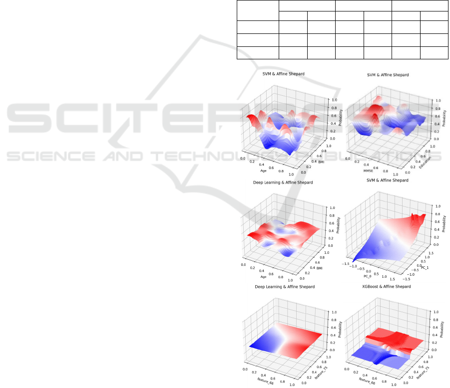
Table 1: Three ML models’ performance data.

Figure 2: Morphing surfaces on Age-BMI and MMSE-

Education, PCA space, and a random feature space using

ADNI dataset.

Accurac

F1 Score AUC score

ADNI Credi

SVM 0.73 0.62 0.73 0.62 0.89 0.65

XGBoost 0.72 0.68 0.72 0.67 0.88 0.74

DL 0.70 0.60 0.70 0.64 0.88 0.64

A Subspace Projection Based Technique for Visualizing Machine Learning Models

891

We applied three popular but different styled ML

algorithms: Support Vector Machine (SVM) (rbf

kernel with gamma=0.05 and C=5), Extreme

Gradient Boosting (XGBoost) (with learning-

rate=0.1 and max-depth=7), and Deep Learning

(DL). The deep neural networks model has 4 hidden

layers with a dropout 0.5 added after each hidden

layer. The overall prediction accuracies, F1 scores,

and AUC scores for both datasets are given in Table

1. The differences in accuracy and other performance

metrics for the three models are not significant here

as we did not do extensive parameter optimization for

performance purposes

5.3 Visualization

Figure 2 shows the morphing surfaces on various

viewing spaces for the ADNI dataset. Figure 3 shows

the morphing surfaces on two 2D feature spaces for

the Home Credit dataset. It is interesting to see that

SVM and Deep Learning generate smoother surfaces

than XGBoost, maybe because XGBoost is a decision

tree based algorithm. Based on Figure 2, it appears

that people in the late 50

with low BMI and people

in the 80

with high BMI have higher risk of AD. We

also see that education level does not seem to play a

major role, but MMSE score is clearly a strong

indicator of AD risk. In Figure 3, we also see that the

loan default risk is greater for high income and lower

income borrowers outside the normal income range.

It also shows that the home condition does not play a

role in default risk, but loans for purchasing more

expensive goods indicate lower risk of default

Figure 3: Morphing surfaces using Home Credit dataset.

Figure 4 shows several 50 percentile value

surfaces and average value surfaces on both the

datasets. These images mostly confirm the findings

from Figures 2 and 3. In addition, we also see that:

(1) people with higher level education will do slightly

better in lowering AD risks; (2) both older age and

higher BMI level are risk factors for AD; (3) higher

loan amount leads higher risk of default; and (4) very

high and very low income levels lead to higher risks

for default. The results from different models are not

all consistent. This also suggests that visualizing ML

models from different ML algorithms may help us

identify potential errors in some of the models.

Figure 5 shows the 25% and 50% cross-sections

of the histogram distributions over the range of

predicted values. Here we see that XGBoost have

more low (25%) probability values in higher MMSE

score area, but more 50% probability values in low

MMSE score area, indicating that the probability of

AD risk increases as MMSE score decreases

Figure 4: Some examples of 50 percentile and average

value visualizations using both datasets.

IVAPP 2025 - 16th International Conference on Information Visualization Theory and Applications

892

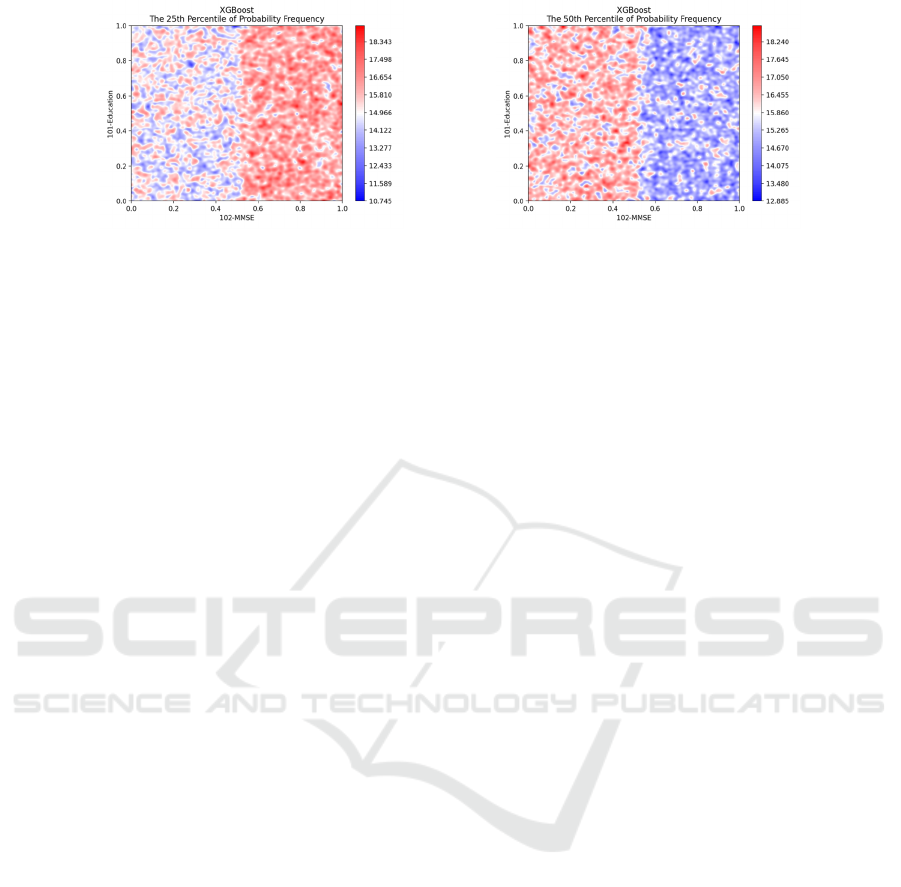
Figure 5: Cross-sections at 25% and 50% for the histogram volumes on the MMSE-Education space using the ADNI dataset.

6 CONCLUSIONS

We have presented a new technique for visualizing

ML models generated from supervised single valued

ML algorithms. While visualization of ML processes

is important for users to understand the decision-

making process, it is often as important to provide a

visual representation of the entire model to gain a

high-level understanding about how the model

behaves in different viewing spaces. Our approach

differs from traditional higher dimensional data

visualization as we aim to represent the global shape

information of the model which is considered a

manifold in a high-dimensional space. In addition,

this type of model visualization techniques has the

potential to become an essential component for visual

interactions in an interactive ML system or human-

in-the-loop AI system. For example, model

visualization can be used as an interface for users to

decide what actions need to be taken to incrementally

improve the model, for example, by adding additional

training samples.

In the future, we would like to extend the

subspace project technique to handle non-linear

subspaces and more complex subspace sampling and

filtering methods. We would also like to develop a

robust user interface to allow interactive exploration

of the different visualization options and

perspectives

REFERENCES

Adadi A, Berrada M. (2018). Peeking inside the black-box:

a survey on explainable artificial intelligence (XAI).

IEEE Access 2018; 6: 52138–52160

Angelos Chatzimparmpas, Rafael M. Martins, Ilir Jusufi,

and Andreas Kerren. (2020). A survey of surveys on the

use of visualization for interpreting machine learning

models. Information Visualization. Volume 19, Issue 3,

July 2020, Pages 207-233.

Seifert C, Aamir A, Balagopalan A, et al. (2017).

Visualizations of deep neural networks in computer

vision: a survey. In: Cerquitelli T, Quercia D, Pasquale

F (eds) Transparent data mining for big and small data.

Cham: Springer, 2017, pp. 123–144.

Liu S, Maljovec D, Wang B, et al. (2017). Visualizing high-

dimensional data: advances in the past decade. IEEE T

Vis Comput Gr 2017; 23(3): 1249–1268

Kaufman, A. (1992). Fundamentals of Volume

Visualization. In: Kunii, T.L. (eds) Visual Computing.

CG International Series. Springer, Tokyo.

https://doi.org/10.1007/978-4-431-68204-2_16.

Endert A, Ribarsky W, Turkay C, et al. (2017). The state of

the art in integrating machine learning into visual

analytics. Comput Graph Forum 2017; 36(8): 458–486

May T, Bannach A, Davey J, et al. (2011). Guiding feature

subset selection with an interactive visualization. In:

Proceedings of the 2011 IEEE conference on visual

analytics science and technology (VAST), Providence,

RI, 23–28 October 2011, pp. 111–120. New York:

IEEE.

Zahavy, T., Ben-Zrihem, N., Mannor, S. (2016). Graying

the black box: Understanding dqns. In: ICML pp.

1899–1908.

Rauber, P.E., Fadel, S., Falcao, A., Telea, A. (2017).

Visualizing the hidden activity of artificial neural

networks. IEEE TVCG 23 (1), 101–110.

Tzeng, F.Y., Ma, K.L. (2005). Opening the black box - data

driven visualization of neural networks. In: IEEE

Visualization, pp. 383–390. http://dx.doi.org/10.1109/

VISUAL.2005.1532820.

Harley, A.W. (2015). An interactive node-link

visualization of convolutional neural networks. In:

International Symposium on Visual Computing.

Springer, pp. 867–877.

Streeter, M.J., Ward, M.O., Alvarez, S.A. (2001). Nvis: An

interactive visualization tool for neural networks.

Liu, M., Shi, J., Li, Z., Li, C., Zhu, J.J.H., Liu, S. (2017).

Towards better analysis of deep convolutional neural

networks. IEEE TVCG 23 (1), 91–100.

http://dx.doi.org/10.

Jason Yosinski, Jeff Clune, Anh Nguyen, Thomas Fuchs,

and Hod Lipson. (2015). Understanding Neural

Networks Through Deep Visualization. ICML

Workshop on Deep Learning, 2015.

A Subspace Projection Based Technique for Visualizing Machine Learning Models

893

Luisa M Zintgraf, Taco S Cohen, Tameem Adel, Max

Welling. (2017). Visualizing Deep Neural Network

Decisions: Prediction Difference Analysis.

International Conference on Learning Representations

(ICLR) 2017.

SeungJin Lim. (2014). A Light-Weight Visualization Tool

for Support Vector Machines. 25th International

Workshop on Database and Expert Systems

Applications, 2014.

Lutz Hamel, (2006). Visualization of Support Vector

Machines with Unsupervised Learning, IEEE

Symposium on Computational Intelligence and

Bioinformatics and Computational Biology, 2006.

Wang, J; Fang, S; Li, H; Goni, J; Saykin, AJ; Shen, L.

(2016). Multigraph Visualization for Feature

Classification of Brain Network Data. EuroVis

Workshop on Visual Analytics (EuroVA), pp.61-65,

2016.

Ren, D., Amershi, S., Lee, B., Suh, J., Williams, J.D.

(2017). Squares: Supporting interactive performance

analysis for multiclass classifiers. IEEE TVCG 23 (1),

61–70.

Alsallakh, B., Hanbury, A., Hauser, H., Miksch, S., Rauber,

A. (2014). Visual methods for analyzing probabilistic

classification data. IEEE TVCG 20 (12), 1703–1712.

Chuang, J., Gupta, S., Manning, C.D., Heer, J. (2013).

Topic model diagnostics: Assessing domain relevance

via topical alignment. In: ICML, pp. 612–620.

Jiawei Zhang, Yang Wang, Piero Molino, Lezhi Li and

David S. Ebert. (2019). Manifold: A Model-Agnostic

Framework for Interpretation and Diagnosis of

Machine Learning Models. IEEE Transactions on

Visualization and Computer Graphics, 25(1), 2019, pp

364 – 373.

H. Li, S. Fang, S. Mukhopadhyay, A. J. Saykin and L. Shen.

(2018). Interactive Machine Learning by Visualization:

A Small Data Solution. IEEE International Conference

on Big Data (Big Data), Seattle, WA, USA, 2018, pp.

3513-3521, doi: 10.1109/BigData.2018.8621952

Liu, Shusen & Wang, B. & J. Thiagarajan, Jayaraman &

Bremer, Peer-Timo & Pascucci, Valerio. (2015). Visual

Exploration of High-Dimensional Data through

Subspace Analysis and Dynamic Projections.

Computer Graphics Forum. 34. 10.1111/cgf.12639.

Chiu, Chia-Hsing, et al. (2020). Human-in-the-loop differen-

tial subspace search in high-dimensional latent space.

ACM Transactions on Graphics (TOG) 39.4: 85-1.

Gerber, Samuel, et al. (2010). Visual exploration of high

dimensional scalar functions. IEEE transactions on

visualization and computer graphics 16.6: 1271-1280.

Shiaofen Fang, R. Srinivasan, Raghu Raghavan and Joan

Richtsmeier. (2000). Volume Morphing and Rendering

-- An Integrated Approach. Journal of Computer Aided

Geometric Design, 17(1):59-81, January, 2000.

Cook, P., Bai, Y., Nedjati-Gilani, S., Seunarine, K., Hall,

M., Parker, G. and Alexander, D. (2006). Camino:

open-source diffusion-mri reconstruction and

processing. 14th Scientific Meeting of the International

Society for Magnetic Resonance in Medicine, Vol.

2759, Seattle WA, USA.

IVAPP 2025 - 16th International Conference on Information Visualization Theory and Applications

894