The Devil Lies in the Details for Species Coexistence Stability in Ablated

and Unablated Five-Species Evolutionary Spatial Cyclic Games

Dave Cliff

School of Engineering Mathematics and Technology, University of Bristol, Bristol BS8 1UB, U.K.

Keywords:

Agent-Based Mode Biodiversity, Cyclic Competition, Asymmetric Interaction, Species Coexistence,

Evolutionary Spatial Games, Rock-Paper-Scissors-Lizard-Spock, Replication.

Abstract:

I present exploration of key results from the series of ablated ﬁve-species “Rock-Paper-Scissors-Lizard-Spock”

minimal agent-based evolutionary models of biodiversity introduced by Zhong, Zhang, Li, Dai, & Yang in their

2022 paper “Species coexistence in spatial cyclic game of ﬁve species” (Chaos, Solitons and Fractals, 156:

111806). At the heart of Zhong et al.’s model of ecosystems coexistence is the Elementary Step (ES) algorithm

in which one or two neighboring agents are chosen at random to engage in one or more interactions selected

at random from the set {COMPETE, REPRODUCE, MOVE}. Minor revisions to the ES algorithm have recently

been introduced to make it more computationally efﬁcient in space and in time, and one contribution of this

paper is to demonstrate that switching to this “Revised ES” (RES) has the unexpected effect of totally changing

the outcomes of Zhong et al.’s simulation experiments. I present analysis of the RES-based experiments which

shows that the key difference is that in RES the likelihood of an agent moving is decoupled from the likelihood

of an agent reproducing or competing, whereas in the original ES the likelihoods of the three possible actions

are interdependently coupled. The fact that such relatively minor changes to the ES algorithm result in such

major changes in the experiment outcomes casts signiﬁcant doubt on the extent to which results such as those

from Zhong et al.’s original experiments can be trusted as truly representative of the real-world biological

systems that they are supposedly intended to model. Python source-code available on GitHub can be used to

replicate the results presented here.

1 INTRODUCTION

1.1 Evolutionary Spatial Cyclic Games

There is a long tradition of empirical bioinformatics

research exploring issues in ecosystems biodiversity,

and speciﬁcally in the population dynamics of species

co-existence, by running sets of computer simulation

experiments of minimal models of multiple interact-

ing species in what are known as Evolutionary Spatial

Cyclic Games (ESCGs). In these simulated systems,

each individual agent (i.e., each modelled organism)

in the population can move (i.e., each agent i occu-

pies a speciﬁc position in space at time t, denoted

by ⃗p

(t), and it may move to some different location

later in time such that ⃗p

(t + ∆

) ̸= ⃗p

(t)). Neighbor-

ing agents in these models may compete in pairwise

ﬁght-to-the-death predator/prey interactions, in which

the loser dies leaving an empty space; and any empty

https://orcid.org/0000-0003-3822-9364

space may subsequently be ﬁlled with a new agent,

created by reproduction, asexually spawning a clone

of a neighboring living agent into the empty spot.

Inspired by the work of (May and Leonard, 1975),

the complexities of real-world predator-prey inter-

actions are reduced in these models to very simple

two-player competitive games that require almost no

time to simulate, and to give interesting coevolution-

ary population dynamics the game is usually cyclic,

i.e. it has intransitive dominance relationships. The

most well-known of such cyclic games is the hand-

gesture game Rock-Paper-Scissors (RPS): Rock beats

Scissors; Scissors beats Paper; and Paper beats Rock.

Using RPS as the predator-prey game allows for the

study of three-species model ecosystems (i.e., where

there are three species denoted by s

, s

, and s

, with

individuals in species s

always playing Rock, etc).

Despite their abstract simplicity, RPS-based

ESCGs have been useful in explaining aspects of

real-world biological systems in which such cyclic

dominance relationships do occur and are sustained:

Cliff, D.

The Devil Lies in the Details for Species Coexistence Stability in Ablated and Unablated Five-Species Evolutionary Spatial Cyclic Games.

DOI: 10.5220/0013132500003911

Paper published under CC license (CC BY-NC-ND 4.0)

In Proceedings of the 18th International Joint Conference on Biomedical Engineering Systems and Technologies (BIOSTEC 2025) - Volume 1, pages 545-554

ISBN: 978-989-758-731-3; ISSN: 2184-4305

545

Figure 1: Dominance network digraphs for Rock-Paper-

Scissors (RPS: left) and for Rock-Paper-Scissors-Lizard-

Spock (RPSLS: right). In both digraphs, the N

different

species S

are denoted by nodes labelled with index i ∈

{1,...,N

−1}, with arcs (directed edges) running from the

dominator (“predator”) species to the dominated (“prey”’)

species. The rules of RPSLS are: scissors cut paper; pa-

per covers rock; rock blunts scissors; scissors decapitates

lizard; lizard eats paper; paper disproves Spock; Spock va-

porizes rock; rock crushes lizard; lizard poisons Spock; and

Spock smashes scissors.

for examples, see the various papers cited in (Nag

Chowdhury et al., 2023).

An extension of RPS

to a ﬁve-gesture cyclic game known as Rock-Paper-

Scissors-Lizard-Spock (RPSLS) was introduced by

(Kass and Bryla, 1998) and that game has since been

widely used to study ﬁve-species model ecosystems.

Groundbreaking papers in this ﬁeld of study were

published over the period 2006-2008: see, for exam-

ple, (Laird and Schamp, 2006; Reichenbach et al.,

2007a; Reichenbach et al., 2007b; Laird and Schamp,

2008; Reichenbach et al., 2008)

This current paper presents results from ESCG ex-

periments where one or more of the dominance re-

lationships in the RPSLS game have been removed,

giving rise to systems that I refer to as ESCGs with

ablated dominance networks.

1.2 Ablated Dominance Networks

Let N

denote the number of species in the ESCG

model. The intransitive predator/prey dominance re-

lationships of the N

=3 RPS and N

=5 RPSLS games

are illustrated as directed graphs (or digraphs) in Fig-

ure 1. Such digraphs are referred to here as domi-

nance networks.

In a recent paper, (Zhong et al., 2022) explored the

effects of selectively ablating one or more relation-

ships from the RPSLS dominance network. That is,

Zhong et al. deleted one or more of the arcs (directed

edges) from the RPSLS digraph, and then observed

the frequency distribution of asymptotic experiment

outcomes from large numbers of independent and

These include (Jackson and Buss, 1975; Sinervo and

Lively, 1996; Durrett and Levin, 1998; Elowitz and Leibler,

2000; Kerr et al., 2002; Gilg et al., 2003; Lankau and

Strauss, 2007; Nahum et al., 2011) and (Guill et al., 2011).

identically distributed (IDD) runs of the ESCG sim-

ulator using the ablated dominance network. Here,

“asymptotic” is interpreted in its usual sense, of the

response of the system as time t→∞, and the ex-

periment outcomes of interest are the number of co-

existing species at the end of the experiment. If we

let T denote the pre-speciﬁed experiment end-time

(where T is assumed to be sufﬁciently big that the

system does indeed settle to its asymptotic state), and

if we let n

(t) denote the number of species in the

system still surviving at time t, then the key observa-

tions in Zhong et al.’s study was the set of frequencies

F(n

(T )=c) : c ∈ {0,1,.. .N

Zhong et al. studied the effect of varying the mo-

bility parameter in the ESCG (denoted by M, and ex-

plained in more detail in Section 2), which deter-

mines how mobile the individual agents are, and for

each ablated dominance network they plotted graphs

of F(n

(T )=c) as a function of M. Zhong et al. re-

ported a diversity of experiment outcomes, depending

on exactly which arc or arcs had been ablated from the

RPSLS dominance network. Section 2 summarises

the work of Zhong et al. in more detail.

In (Cliff, 2024b) I presented results which repli-

cated and conﬁrmed Zhong et al.’s results, before

questioning whether they had chosen a sufﬁciently

large valure of T for their simulations to truly con-

verge on asymptotic states. In this paper I go

on to fully explore the effects of re-running Zhong

et al.’s experiments with a slightly different style

of ESCG simulation recently introduced in (Cliff,

2024a), which involves what are prima facie only

very minor adjustments to the core algorithm in the

ESCG simulation, the so-called Elementary Step (ES).

The initial motivation for altering the ES was to im-

prove its efﬁciency in space and in time. The revised

algorithm and associated initial results were ﬁrst pub-

lished in (Cliff, 2024a), a paper presented at an in-

ternational conference on modeling and simulation

methods, where the focus was on the computational

efﬁciency increases (reductions in execution time for

the simulations) and where I did not seek to explore

the effects of using the revised ES algorithm across

the full range of ablated dominance-network species

co-existence experiments reported by Zhong et al..

My new results and analysis presented here show

that switching from the “Original” Elementary Step

(OES) used by (Zhong et al., 2022) to the “Revised”

Elementary Step (RES) introduced in (Cliff, 2024a)

has a major effect on every single one of the key ex-

periment outcomes reported in (Zhong et al., 2022);

that is, for all of Zhong et al.’s key results, I demon-

strated in (Cliff, 2024b) that they can be replicated

very well with OES and then in this paper, when I

BIOINFORMATICS 2025 - 16th International Conference on Bioinformatics Models, Methods and Algorithms

546

switch the simulator to instead use RES, I get to-

tally different outcomes – identifying and explaining

that difference is the key contribution of this paper.

The Python source-code initially developed for the

research reported in (Cliff, 2024a) is freely-available

public-domain open-source software on GitHub,

I give further details of the OES-based ESCG as

used by Zhong et al. (and many other researchers) in

Section 2, and then explain the differences between

OES and RES in Section 3. I discuss differences be-

tween OES and RES results in Section 4. Then in

Section 5 I explain the root cause of those differences

and discuss the extent to which they cast doubts on

just how far results from OES can be trusted as being

representative of the real-world biosystems that they

are intended to be informative models of.

2 THE ESCG ALGORITHM

Zhong et al. used the de facto standard algorithm for

their Evolutionary Spatial Cyclic Game (ESCG), the

core elements of which were established in (Reichen-

bach et al., 2007a).

The position ⃗p

of each individual agent i in the

population is represented by the values on a Cartesian

lattice l of some dimensionality, and almost all work

in this ﬁeld studies systems where the lattice is a 2-

dimensional square of side-length L, so the maximum

total population size is N=L×L, where the position ⃗p

of an individual agent i can be represented by an (x,y)

row-column co-ordinate pair indexing into the lattice

as l(x,y). Cells (or ‘positions’ or ‘locations’) in the

lattice can be empty, denoted here by

0, or they can be

occupied by a single individual agent. In the RPSLS-

based systems explored by (Zhong et al., 2022), the

number of species is ﬁxed at N

=5, and the species

identiﬁer indexes will here run 0,. .., N

− 1, so the

set of possible lattice cell-values is C

= {

0,0,. .. ,4}.

Let U(S) denote the uniform (equiprobable) ran-

dom choice of a member from set S, and let U[n

]

denote a fresh random draw from a uniform distri-

bution over the range [n

] ⊂ R. To initialise

the lattice, some researchers include a number of

empty cells in the initial state, but (Zhong et al.,

2022) do as many other authors do, starting in-

stead with every cell containing an agent, with each

species s

being chosen with probability

∀i such

that l(x, y)=U({0, ... ,4})∀(x, y).

The ESCG is then simulated as a simple discrete-

time system. At the core of the simulation is the El-

ementary Step (ES), the original and revised forms

See github.com/davecliff/ESCG Python

of which (i.e., the OES and RES) are discussed fur-

ther in Section 3. In both the OES and the RES, the

ES implements an interaction between two randomly-

chosen neighboring cells, and this requires the re-

searcher to commit to a neighborhood function and

to a speciﬁc boundary condition. The neighborhood

function is typically either the von Neumann or the

Moore. The boundary condition is typically either

periodic, where the square lattice is, topologically, a

toroidal surface; or no-ﬂux, where the edges of the lat-

tice are hard boundaries on a ‘walled garden”. Zhong

et al. used the von Neumann Neighborhood and no-

ﬂux boundary conditions, and so that is what I used

in the replication experiments described here.

Implementing the random selection of a cell and

its randomly chosen neighbor is trivial. Once two

neighboring cells have been chosen, they may inter-

act, and the opportunity set of possible interactions is

the same for both OES and RES:

• If both cells contain agents, they might compete

according to the rules of the ESCG’s dominance

network for species-to-species interactions. Com-

petition will result either in a draw (no change), or

the dominated ‘prey’ individual dies and the lat-

tice cell it was occupying is replaced by

• If one cell contains an agent and the other contains

0 (i.e., is empty), the agent might reproduce by

cloning a copy of itself into the empty cell.

• The contents of the two cells might be swapped,

which implements a one-step move for each of the

two cells’ contents.

Which, if any, of these three interactions occurs

on any one ES is determined stochastically, and the

random choice of interaction is determined by three

system hyperparameters: µ, which primarily affects

the probability of choosing compete; σ, which primar-

ily affects the probability of choosing reproduce; and

ε which primarily affects the probability of choosing

move. Zhong et al. describe these three as “probabil-

ities” but (as is explained below in Section 3) this is

incorrect: they are relative interaction rates.

The convention in this ﬁeld of research is to talk of

time-steps at two levels of granularity: the ES is the

ﬁner-grained time-step, but it involves only a single

potential interaction between two randomly chosen

cells in what is usually a large lattice of such cells. At

a coarser-grained level, researchers talk of the Monte

Carlo Step (MCS) as being the primary unit of time,

a time-step in which all N cells in the lattice can po-

tentially experience at least one interaction: i.e., one

MCS involves N elementary steps being executed.

In all the experiments they reported in detail,

Zhong et al. used L=200 and (in common with many

The Devil Lies in the Details for Species Coexistence Stability in Ablated and Unablated Five-Species Evolutionary Spatial Cyclic Games

547

other researchers) they set µ=σ=1.0 for all experi-

ments, stating that they did so without loss of gener-

ality. Following the de facto standard procedure es-

tablished in many prior papers in this ﬁeld, Zhong et

al. did not explicitly set values for the movement fac-

tor ε, but instead systematically varied, as the primary

independent variable in their experiments, a mobility

parameter M, which relates the movement rate ε to

the lattice size N via ε=2MN. For each of their key

experiments, Zhong et al. varied M in discrete steps

over M∈[10

−7

,10

−3

], sampling the response of the

system, its frequency distribution of ﬁnal outcomes, at

each M-value. At each value of M sampled, Zhong et

al. performed N

IID

=500 independent and identically

distributed (IID) simulation experiments.

Finally, to complete the speciﬁcation for one of

the RPSLS-style ESCGs simulated by (Zhong et al.,

2022), the dominance network needs to be deﬁned. In

(Cliff, 2024b) I introduced terminology to distinguish

the various ablated RPSLS dominance networks that

Zhong et al. explored (each of which, Zhong et al. re-

ferred to solely by reference to which ﬁgure-number

in their paper the relevant network diagram appeared

in): let Z0 denote the original unablated RPSLS net-

work as illustrated in Figure 1, and then let any ver-

sion of that network with n

arcs ablated be referred

to as a Zn

network, so for example Z0 with two ab-

lated arcs would be referred to as a Z2 network; then

in the cases where Zhong et al. studied two topologi-

cally nonisomorphic networks of type Zn

, add qual-

ifying letters a and b as sufﬁxes. In total, Zhong et

al. studied the dynamics of ESCGS with six different

ablated versions of Z0, referred to as Z1, Z2a, Z2b,

Z3a, Z3b, and Z4; for full details, see (Cliff, 2024b).

The ESCG algorithm used by Zhong et al. is sim-

ple to describe: the 2D lattice L is randomly initialised

at t=0, as described above, and the dominance net-

work D is set up. An outer time-step loop iterates

over each MCS, within which an inner loop iterates

N times over the Elementary Step (ES) procedure

ELSTEP. After each MCS time-step, the population

density of each of the N

species (denoted by ρ

for

i ∈ {0,.. .,N

− 1}), along with the density of empty

cells (denoted by ρ

) is recorded, optionally along

with the state of the lattice at that MCS. At the end

of each IID simulation run, the time-series of densi-

ties ρ

and ρ

∀i are written to an output ﬁle, and the

set of frequency distributions of experiment outcomes

(i.e., F(n

(T )=c) for c ∈ {1,. .., 5}) are updated. The

ﬁnal Fs for the set of N

IID

simulations is, in the cur-

rent context, the primary data of interested returned

by the ESCG.

The elementary step (ES) algorithm ELSTEP is

similarly straightforward. It is trivial to randomly

choose a cell in the lattice, and to randomly choose

a neighbor of that cell given the pre-deﬁned neigh-

borhood function and boundary conditions. Imple-

menting the three individual cell-to-cell interaction

procedures COMPETE, REPRODUCE, and MOVE is

similarly unproblematic. However, to better facili-

tate the comparison between OES and RES, there is

some subtlety required in describing the method for

randomly selecting the interaction(s) to be enacted on

any one elementary step: here we’ll assume that EL-

STEP can call a function GET3PR which returns three

interaction probabilities P

∗

, and P

∗

that respec-

tively set the likelihood of ELSTEP calling COMPETE,

REPRODUCE, and MOVE. This can be simply imple-

mented by generating three random real values r

each via U[0,1], and then executing COMPETE if

< P

∗

; executing REPRODUCE if r

< P

∗

; and exe-

cuting MOVE if r

< P

∗

. For OES, GET3PR always

returns two of the three probabilities as zero, and the

other probability as one – this ensures that only one

of the three possible interactions occurs on any one

elementary step, which is the convention introduced

in the seminal papers of (Reichenbach et al., 2007a);

a convention that has been continued in all published

literature that replicates and builds upon those works.

The calculation of the three interaction probabili-

ties is where the revised elementary step (RES) differs

from the original elementary step (OES), and that is-

sue is discussed in more detail in the next section.

3 OES vs. RES

The difference between the OES, used by (Zhong

et al., 2022) and many others,

and the RES, intro-

duced in (Cliff, 2024a), boils down to how the three

probabilities used in ELSTEP, P

∗

, and P

∗

, are cal-

culated from the interaction rates µ, σ, and ε. Be-

cause we’re repeatedly dealing here with triplets of

values, let

⃗

R = (µ,σ, ε) denote the vector of inter-

action rates; let

⃗

∗

) = (P

∗

),P

∗

),P

∗

))

denote the vector of interaction probabilities at time

, measured here at the micro-level of the count

of individual elementary steps, rather than the macro

level of MCS-number; and let

⃗

P = (P

) denote

The core of OES can be traced back to (Gillespie,

1976), cited approvingly in the landmark paper of (Reichen-

bach et al., 2007a). Other authors who have reported re-

sults from OES-based studies include (Nagatani et al., 2018;

Kabir and Tanimoto, 2021; Mood and Park, 2021; Park,

2021; Avelino et al., 2022; Bazeia et al., 2022; Menezes

et al., 2022a; Menezes et al., 2022b; Zhang et al., 2022;

Park and Jang, 2023; Menezes et al., 2023); and (Kubyana

et al., 2024).

BIOINFORMATICS 2025 - 16th International Conference on Bioinformatics Models, Methods and Algorithms

548

the vector of normalized probabilities, explained fur-

ther below.

The OES method, which is the de facto standard

method in ESCG modelling, can be traced back to ﬁrst

usage in the landmark papers of (Laird and Schamp,

2006) and (Reichenbach et al., 2007a). In those origi-

nal sources, each of the elements of

⃗

R clearly have the

potential to take on values greater than one.

However, quite often the three interaction rates

have since been described by other authors of papers

using OES as being bounded to the range [0.0,1.0]

and are also referred to by several authors as ‘prob-

abilities’, despite the fact that they are not actually

treated as literal probabilities: for example, µ = 0.5

does not necessarily mean there is a 50% chance of

COMPETE being the next interaction: it might do, and

it might not, depending on the contemporaneous val-

ues of σ, and ε. This is because the three interac-

tion rates are ﬁrst subjected to a normalization pro-

cess that divides each of the three by the sum of the

three, giving three “normalized probabilities” P

and P

, the elements of

⃗

P, which are each within [0,1]

and which collectively sum to one.

To understand this, the values for the interac-

tion rates µ, σ, and ε can be thought of in OES as

indications for what relative proportion of a three-

segment roulette-wheel is allocated to each possi-

ble interaction, and then in the OES the concep-

tual roulette-wheel is spun once, generating a ran-

dom value r(t

)=U[0.0, 1.0], which is then com-

pared to the elements of

⃗

P such that the interaction

at t

will be COMPETE if 0 ≤ r(t

) < P

; REPRO-

DUCE if P

≤ r(t

) < P

+ P

; and MOVE other-

wise (because P

= 1.0 − (P

+ P

)). This method is

widely known as roulette selection in the literature on

evolutionary computation (see e.g. (Lloyd and Amos,

2017)). Hence, with OES,

⃗

∗

) is always either

(0,0,1) or (0,1, 0) or (1,0, 0), roulette-selected on the

basis of

⃗

P and r(t

): i.e., only one randomly-chosen

type of interaction can ever happen per single OES.

The corresponding calculation in RES is much

simpler to explain because the interaction rates µ and

σ are interpreted instead as actual probabilities, de-

ﬁned only over [0,1], and mapping directly (via the

identity function) onto P

∗

and P

∗

, respectively; the

movement rate ε is required to be non-negative and is

interpreted as mapping directly onto P

∗

, with the sim-

ple ﬁlter that if ε>1.0 then it is capped to one. Thus

in RES there is no

⃗

P and instead an essentially direct

mapping from

⃗

R to

⃗

∗

). This means that, whereas

in OES there is a constraint that |

⃗

∗

)|=1 ∀t

, in

RES instead |

⃗

∗

)| ∈ [0, 3] ∈ R – i.e., at the limit,

⃗

∗

)=(1,1,1) is perfectly well deﬁned.

On the face of it, the change between OES and

RES is pretty minimal. Whereas OES’s roulette-

selection means that only one interaction can oc-

cur per ES, the deﬁnition of RES allows up to

three interactions to occur per ES. For example,

if µ=σ=ε=1.0 (i.e.,

⃗

R=(1,1,1)) then in OES one

of the three possible actions will be randomly

chosen, using r(t

) and

⃗

P=(

), and then

⃗

∗

) ∈ {(1,0,0), (0,1,0),(0,0, 1)} depending on

r(t

); whereas in RES, for the same

⃗

R we have

⃗

∗

⃗

R=(1,1,1) and hence, whenever possible,

on each RES there will be a call to COMPETE, fol-

lowed by a call to REPRODUCE, followed by a call to

MOVE. This means that, when

⃗

R=(1,1,1), if possi-

ble a single agent can, in one RES, kill its neighbor-

ing opponent in COMPETE, and then REPRODUCE a

clone of itself into the

0-cell just vacated by the dead

opponent; and then MOVE into the neighboring cell,

swapping position with its newly-spawned offspring.

Whereas with OES the same agent would engage in

at most one randomly-chosen interaction per ES, and

so would require three consecutive ESs to achieve the

same sequence of events.

For that reason, one might expect a RES-based

replication of any of the experiments reported in

(Zhong et al., 2022) to proceed up to three times faster

than the comparable OES-based experiment – and in-

deed it was a desire for reduced run-times that moti-

vated the development of RES, as reported in (Cliff,

2024a), where further analysis and discussion of the

speed-up enabled by RES is given. Here, the focus is

not on the run-times of the simulations, but instead on

the unexpected results that I report in the next section:

the outcomes of every single one of Zhong et al.’s ab-

lation experiments is dramatically altered when the

ES is switched from OES to RES, an unexpected con-

sequence of RES that was not explored in any depth

in (Cliff, 2024a).

4 RESULTS

4.1 Original Elementary Step (OES)

As with the original results of (Zhong et al., 2022)

and also with my replication of those results reported

in (Cliff, 2024a), in all the experiments I discuss in

(Cliff, 2024b) I set T =10

MCS, L=200, µ=σ=1.0,

and ranged M from M

min

=10

−7

to M

max

=10

−3

, us-

ing a multiplier of 10

1/5

to give ﬁve sampled M data-

points per order of magnitude, and I ran OES-based

simulation experiments for all six of Zhong et al.’s

networks Z1, Z2a, Z2b, Z3a, Z3b, and Z4 – the com-

plete set. All my results presented in (Cliff, 2024b)

The Devil Lies in the Details for Species Coexistence Stability in Ablated and Unablated Five-Species Evolutionary Spatial Cyclic Games

549

agree very well with the original results of (Zhong

et al., 2022).

In each set of experiment outcomes the key ob-

servable feature, as highlighted by Zhong et al., is

a sudden transition part-way between M=10

−5

and

M=10

−4

from three-or-more-species coexistence be-

ing the dominant outcome, to two or fewer coexisting

species always being the outcome – i.e., a “collapse”

in ecosystems diversity. If this result is general, i.e.

if it is applicable to real-world ecosystems and is not

just an artefact of the particular details of Zhong et

al.’s ESCG modelling methods, then surely we should

expect to see it also when the only change made to the

ESCG is to switch from OES to RES – and in fact, if

anything, we should expect to see the collapse sooner

(after a shorter T ) when working with RES, because

of its potential for a three-times speed-up.

4.2 Revised Elementary Step (RES)

For my RES experiments, I swept M within the range

[5×10

−8

,1.25×10

−5

] to give the same range of P

values as were used by (Zhong et al., 2022) in their

OES experiments.

To avoid what would otherwise surely be a strong

contender for the most boring set of graphs ever pub-

lished in a scientiﬁc paper, here I give only verbal de-

scriptions of the outcomes of my RES-based replica-

tions of Zhong et al.’s experiments. I only need to de-

scribe two outcomes because my results were unam-

biguously bimodal: for networks Z0, Z2b, Z3b, and

Z4, the FvsM outcome was essentially identical: the

system never deviated from F(n

(T )=5)=1.0 across

the entire range of M values; and for the remaining

networks (i.e., Z1, Z2a, and Z3a) the outcome was

again essentially identical, but in these three cases

the system’s asymptotic state was F(n

(T )=3)=1.0

across the entire range of M values. That is, in all my

RES experiments, the outcome at T was always ei-

ther three-species coexistence or ﬁve-species coexis-

tence, for every network studied by Zhong et al.: that

is, once you switch to RES, the collapse in ecosystems

diversity seen every time when using OES simply dis-

appears.

And yet that switch, from roulette-selecting a sin-

gle interaction in OES to probabilistically selecting

one, two, or three interactions in RES, seems only a

very small change, a mere implementation detail in-

tended to speed things up a bit – the set of possible

interactions remains unchanged, so why does RES

result in such different outcomes to OES? And, un-

less it can be convincingly argued that OES is some-

how a better representation, a better abstraction, of the

natural world than is RES, then surely this fragility,

these major changes in outcomes resulting from mi-

nor changes to the internal mechanisms, casts signif-

icant doubt on the generality and applicability of the

OES-based results published by (Zhong et al., 2022),

and indeed of the results in any other published pa-

pers (and there are many) that show results from OES-

based ESCGs. This discrepancy in the results is dis-

cussed in more detail in the following section.

5 DISCUSSION

To understand why the RES outcomes differ so

markedly from the OES ones, it is necessary to go

back and consider the step in OES where the three

system hyperparameters, the interaction rates µ,σ,

and ε, are ‘normalized’ to give internal probabilities

, and P

prior to the roulette-selection of a sin-

gle action for that ES. The normalization process in-

tertwines the three rates, and they cease to be indepen-

dent, and yet this seems to be rarely if ever acknowl-

edged in the literature.

For example, sweeping M across a range such as

the [10

−7

,10

−3

] used by Zhong et al., is described

by Zhong et al. (and by many other authors who also

present results from parameter-sweeps on M, this be-

ing a common way of exploring ESCGs) as systemat-

ically varying mobility, i.e. treating M as the indepen-

dent parameter in the experiments. While altering M

deﬁnitely does alter the likelihood of movement for

the agents in the ESCG, in OES it also alters the like-

lihood of competition, and of reproduction. Specif-

ically, in OES, increasing mobility M increases the

probability of movement P

, but it can also decrease

the probabilities of competition (P

) and reproduction

). Figure 2 shows the changes in values of the

three probabilities over the range of M values used

by (Zhong et al., 2022), all at L=200, for various val-

ues of µ and σ including the µ=σ=1.0 case used by

(Zhong et al., 2022).

As can be seen from the upper left graph in Fig-

ure 2, the µ=σ=1.0 case, as M is increased P

does

indeed rise as intended, but as it rises so P

and P

fall, ending up very close to zero once M≈10

−3

Clearly increasing M not only increases mobility, but

also greatly reduces the frequency of competition

and of reproduction: at M=10

−3

=0.976 while

=0.012; so movement is roughly 80 times

more likely than either reproduction or competition.

In contrast, when using RES, increasing M does in-

deed increase P

, but it has no effect on P

or P

be-

cause the interaction probabilities are independent.

To illustrate this key difference between OES and

RES, Figure 3 shows the unit cube in R

formed by

BIOINFORMATICS 2025 - 16th International Conference on Bioinformatics Models, Methods and Algorithms

550

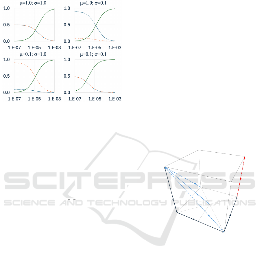
Figure 2: Graphs of the normalized internal probabilities

, P

, and P

for L=200 as calculated in the OES for

M∈[10

−7

,10

−3

], the range used by (Zhong et al., 2022), for

the values of µ and σ shown in each graph title. Each graph

shows plots for P

(dotted line), P

(dash-dot line), and P

(solid line). In all four graphs the horizontal axis is M while

the vertical axis is probability. The upper left graph shows

results from µ=σ=1.0; upper right shows results from

µ=1.0,σ=0.1; lower left shows results from µ=0.1, σ=1.0;

and lower right shows results from µ=σ=0.1.

)-space – a cube that I’ll refer to as “P-

space” hereafter. In Zhong et al.’s OES-based ex-

periments with µ=σ=1.0, As M is swept from 10

−7

to 10

−3

, the three interaction probabilities shift from

their initial point close to (

,0), and move with

nonlinearly varying speed along a straight line in P-

space, to their ﬁnal point at approximately (0,0, 1) –

this is represented by the solid blue arrowed line in

Figure 3. (At L=200, as used by Zhong et al., the ac-

tual start-point is (0.498,0.498, 0.004) and the actual

end-point is (0.01,0.01,0.98)).

However in RES, sweeping M over the corre-

sponding range of values, P

=1.0;∀M, and the

only probability varied as M increases is P

which

rises along the straight line in P-space from its ini-

tial point close to (1,1,0) to its ﬁnal point close to

(1,1,1), which is illustrated by the vertical dashed red

arrowed line in Figure 3.

Because the three interaction probabilities are in-

dependent in RES, one can readily set P

and P

to be

any pair of values in [0, 1]

⊂ R

and then indepen-

dently sweep the mobility M across some range which

maps P

to varying over [0,1] ⊂ R: that is, in RES it

is trivially easy to set up an experiment where the ini-

tial point in P-space is anywhere on the ﬂoor-plane of

the P-space unit cube, and for P

to then range from

zero to one while P

and P

are held constant, giving

a vertical line in P-space. And we need not stop there:

in principle, experiments can be run with RES where

across the duration of the experiment the point in P-

space moves along some arbitrarily-oriented straight

line or curve – there is nothing in RES that limits P

to being the sole independent variable, nothing that

requires only vertical lines in P-space.

However with OES the experimenter’s options are

signiﬁcantly more constrained. To illustrate why this

is so, refer back to Figure 2: the upper left graph

shows the three interaction probabilities versus M for

the case where µ=σ=1.0, and the lower right graph

shows the same three probabilities for µ=σ=0.1; de-

spite the factor of ten difference in the values of µ

and σ between these two graphs, the traces shown

on the graphs are qualitatively very similar: in both

cases, P

and P

both start at ≈0.5 and then decay

sigmoidally to ≈0.0, while P

rises sigmoidally from

≈0.0 to ≈1.0.

To understand this, consider ﬁrst the location of

the start-point in P-space for an OES-based experi-

ment where M is swept from some very small initial

value (like 10

−7

) to some larger ﬁnal value (such as

(0,0,0)

(1,0,0)

(1,1,0)

(1,1,1)

(0,0,1)

(0,1,1)

, P

)

(0,1,0)

Figure 3: Perspective plot of (P

)-space, referred to

here as “P-space”, which is the unit cube [0,1]

⊂R

. The

ﬂoor-plane of the cube is the (P

,0) unit square with,

from this viewpoint, the P

axis running from the origin to

lower-right, and the P

axis running from the origin to up-

per right; the vertical axis is P

. For clarity, seven of the

eight corner vertices are labelled with their coordinates; the

one unlabelled vertex, nearest the viewpoint, is (1,0,1). The

solid blue arrowed line from (0.5,0.5,0.0) to (0,0, 1) shows

the straight-line path of P

values explored by Zhong et al.

in their OES-based experiments as they swept M over the

range [10

−7

,10

−3

] while keeping µ=σ=1.0. The dashed

red arrowed line from (1,1,0) to (1,1,1) shows the straight-

line path of P

values explored when using RES, with M

varied over the corresponding range. The dashed blue ar-

rowed lines starting at (1, 0, 0) and at (0, 1, 0), both ending

at (0,0,1), mark the two vertical-plane edges of the OES

unit 3-simplex: its horizontal edge is the line P

= 1 − P

joining (1,0,0) to (0,1,0): the signiﬁcance of the OES unit

3-simplex is discussed further in the text.

The Devil Lies in the Details for Species Coexistence Stability in Ablated and Unablated Five-Species Evolutionary Spatial Cyclic Games

551

−3

). From the way that the three interaction prob-

abilities are calculated as functions of the three in-

teraction rates in the “normalization” step, whenever

µ=σ, we have P

2µ+ε

. Given that ε=2MN,

when M≪

we have ε≈0 and hence P

≈

2µ

for any case when µ=σ. Thus it is intuitively obvi-

ous that with OES the start-point on the (P

,0)

ground-plane of the P-space unit cube is determined

by the ratio of µ to σ: when µ=σ=c the ratio is 1.0

and the start-point is very close to (0.5, 0.5, 0.0), re-

gardless of the actual value of c; then, as σ/µ → 0,

the start-point moves ever closer to (1,0, 0); and as

σ/µ → ∞ the start-point moves ever closer to (0, 1,0).

And, in the two limit cases, when µ=0 we have P

but P

=σ/(σ+ε) → 1.0 as ε → 0, giving a start-point

of ≈(0, 1,0); and (mutatis mutandis) when σ=0 so

→ 1.0 as ε → 0, giving a start-point of ≈(1, 0,0).

The key thing to note here is that, for any plausible

values of µ and σ, and sufﬁciently low initial value of

M, the start point is always on (or very close to) the

line P

=1 − P

, joining (1,0,0) to (0, 1,0).

Next consider the OES end-point in P-space: this

is easy, it’s always going to be at (or very close to)

(0,0,1), for any plausible values of µ and σ, and suf-

ﬁciently high ﬁnal value of M (i.e., for M ≫

And, taken together, these constraints on the P-

space start-points and end-points for OES-based M-

sweep experiments mean that the set of possible

points sampled in P-space is tightly constrained: the

OES-based experiments are limited to the set of points

on (or very near) the unit 3-simplex (i.e., the planar

triangle deﬁned by the points (1,0, 0), (0,1, 0), and

(0,0,1)); thus, OES experiments are simply not set

up to explore the response of the system in any area

of P-space outside of that three-sided planar area.

To emphasize the importance of this point, let us

consider the expected qualitative asymptotic experi-

ment outcomes at each of the seven corner-vertices of

P-space for which at least one of the interaction prob-

abilities is nonzero, assuming that the ESCG is run

for its duration with the three interaction probabilities

held at the vertex:

• (0, 0, 1): the agents can move, but they never

compete or reproduce, so the whole population of

agents wander aimlessly around the lattice, never in-

teracting with one another. This is a dynamic equi-

librium, but population-level statistics such as species

densities will remain static. There is no chance of

species extinctions with the system at this vertex.

• (0, 1, 0): agents can reproduce, but not move

or compete: any initially empty cells might be ﬁlled

by reproduction, but once there are no empty cells re-

maining the system will have converged to a stasis.

there’s no chance of extinctions at this vertex.

• (1, 0, 0): agents compete, but can’t move or re-

produce: any immediate neighbors in the initial lattice

conﬁguration who are predators/prey will eventually

compete, resulting in the death of the prey. Once all

possible predator/prey interactions in the initial lat-

tice conﬁguration have been resolved by competition,

the number of empty cells will have increased, but

the system will thereafter be at stasis. Species ex-

tinctions can occur when the system is at this vertex:

the likelihood of extinctions is entirely dependent on

the initial distribution of agents on the lattice at t=0.

With uniform random allocation of agents to the lat-

tice positions at t=0 the likelihood of one or more en-

tire species going extinct when the interaction prob-

abilities are held at this vertex is technically nonzero

but will be vanishingly small for any sufﬁciently large

value of L to be of serious interest.

• (0, 1, 1): agents reproduce and move, but don’t

compete: empty cells in the lattice at t=0 will eventu-

ally be ﬁlled by reproduction, and all agents can move

around freely; once the last empty cell is ﬁlled, the

system is thereafter at the same dynamic equilibrium

with static species densities as at vertex (0,0,1), and

so there is no chance of extinctions here either.

• (1, 0, 1): agents compete and move, but don’t

reproduce: the number of empty cells is likely to rise

over the course of the experiment as prey agents are

dominated by predators. Species extinctions are en-

tirely likely when the system is at this vertex, the like-

lihood depending on the dominance network.

• (1, 1, 0): agents compete and reproduce, but

don’t move: the number of empty cells is likely to

rise and fall, with the asymptotic outcome being zero

empty cells. Species extinctions can occur at this ver-

tex, the likelihood depending on l(0) (the state of the

lattice l at t=0) and on the dominance network.

• (1, 1, 1): the whole enchilada – agents can com-

pete, reproduce, and move. Species extinctions can

occur when the system is at this vertex, the likelihood

depending on l(0) and the dominance network.

From this it is clear that, if the ESCG is being run

as a minimal model of ecosystems biodiversity and

species co-existence, the ﬁnal three vertices (1,0,1),

(1,1,0), and (1,1,1) are of primary interest, because

they are the three for which there is a reasonable

chance of species extinctions. These three vertices

are all on the top-plane of the P-space unit cube, and

because none of them are within the unit 3-simplex,

they simply can’t be explored via OES-based mod-

els. Instead, as mobility M is increased in OES-based

models, the system is taken ever-closer to the “aim-

less wandering” P-space vertex (0,0,1).

For example, a naive experimenter might start an

OES M-sweep simulation at µ=1 and σ=0, i.e. at

BIOINFORMATICS 2025 - 16th International Conference on Bioinformatics Models, Methods and Algorithms

552

the (1,0,0) vertex in P-space, and then sweep M over

[10

−7

,10

−3

] in the (mistaken) expectation that this

will increase only P

and eventually take the system

to the (1,0,1) P-space vertex. However the OES nor-

malization process will instead take the system on

a straight-line path toward the (0,0,1) vertex. Some

species extinctions may occur en route, and – as I

have shown in my replication of the results of (Zhong

et al., 2022) — the system will close in on (0,0,1)

but P

and P

can remain nonzero, so extinctions do

remain a possibility. But the OES experimenter’s re-

sults will say nothing about the asymptotic behavior

of the ESCG system at (1,0,1) in P-space: for that,

they would need to abandon OES and switch to RES.

The results from RES-based simulations pre-

sented here show that when areas of P-space that are

unreachable in OES-based simulations are instead ex-

plored via the ESCG with RES, the frequency distribu-

tions of asymptotic experiment outcomes can change

signiﬁcantly. And surely that then calls into ques-

tion the generality and the applicability of the results

from OES-based simulations to the real-world sys-

tems that they are intended as models of: my RES

results present a ﬁrst counter-example to the observa-

tion in OES-based systems of the sudden transition in

experiment outcomes from being n

(T )) ≥ 3 at low

M to n

(T )) ≤ 2 at higher M values: this happens as

the OES-based system converges on P-space vertex

(1,0,0) but does not happen when the RES-based sys-

tem is instead set to converge on (1,1,1).

And from that it seems reasonable to propose that

Zhong et al.’s OES-based results, repeatedly showing

collapses in ecosystems coexistence/diversity as mo-

bility increases, are mere artefacts of their decision to

use OES in their ESCG model: if they’d used RES,

they would have had no story to tell. The only pos-

sible line of counterargument that I can think of here

would be to defend use of OES on the basis that it

is somehow more faithful to ecological reality, more

biologically plausible, than RES, and hence to argue

that OES should continue to be used in preference to

RES because it is, in that sense, the better modelling

method. Now maybe I’m biased in favour of my

own creation, but I’ve tried very hard to think of how

OES could possibly be defended as somehow better

than RES, and thus far I have drawn a blank. The

two methods strike me as equally abstract, equally

(im)plausible approximations to reality, but in OES

the experimenter’s hands are tied in P-space, while

in RES the experimenter can roam freely within the

conﬁnes of that cube, which surely opens up more av-

enues for exploration than repeatedly moving from

the base to the apex of the unit simplex, which is

seemingly the only option with OES. And, in that

sense, arguably RES is a better approximation to re-

ality than OES, because in many real ecosystems it

seems intuitively unlikely that every species’ motil-

ity, fecundity, and likelihood of eating or being eaten

are interdependently bound together by one function

(as in OES), and more likely that these three aspects

of species’ existence are to some extent independently

variable (as in RES). I am of course very open to con-

versation with anyone who wants to argue the point:

discussion and debate is very welcome here.

In this paper I’ve shown results from RES-based

M-sweep experiments where only one path in P-

space, along the line from (1,1,0) to (1,1,1), is ex-

plored. An obvious direction for further work in

attempting to understand these ESCGs as models

of species coexistence and ecosystems biodiversity

would be to generate results from similar RES ex-

periments where the P-space path starts at a different

initial point but still ends at (1,1,1), and also to run

further RES-based simulations that end at (1,1,0) or

(1,0,1), the other two P-space vertices where species

extinctions can be expected to occur at the limit. The

OES-based results can then be judged in the wider

context of comparison to the array of results from the

various RES-based experiments: the extent to which

the sudden shift in n

(T ) outcomes is also seen, if

at all, in the RES experiments will then allow us to

make a reasoned judgement on the generality of that

shift occurring in OES-based outcomes. This is fur-

ther work that I intend to report in one or more forth-

coming papers, but at this stage it seems reasonable

to hypothesize that the M-dependent shift in experi-

ment outcomes seen in the OES systems as reported

by (Zhong et al., 2022) and replicated here is in fact

a mere artefact of the method, a quirk of the OES’s

normalization and roulette-selection process.

6 CONCLUSION

The results presented here offer the ﬁrst clear and

comprehensive set of counterexamples to all the key

results presented by (Zhong et al., 2022), because

I have shown that in the RES-based ESCG experi-

ments, which I contend are just as plausible models

of real-world systems as the OES-based ones, no M-

dependent shift in outcomes (i.e., ﬁnal counts of coex-

isting species) occurs. Provision of these counterex-

amples, and my analysis and explanation in terms of

P-space trajectories, are the contributions of this pa-

per. I see no reason to expect that the problematic

issues identiﬁed here with the use of OES in ESCGS

is limited only to the one paper by Zhong et al. that

I have focused on here. It seems plausible that con-

The Devil Lies in the Details for Species Coexistence Stability in Ablated and Unablated Five-Species Evolutionary Spatial Cyclic Games

553

clusions drawn in many other papers reporting results

from OES-based studies may need to be revised if,

when the same M-sweep experiments are instead run

with a RES-based ESCG, the results come out differ-

ent. Only further work and time will tell, but right

now, from what I’ve presented here, it does seem that

the devil lies in the details for this class of evolution-

ary spatial ecosystem simulation model.

REFERENCES

Avelino, P., de Oliveria, B., and Trintin, R. (2022). Parity

effects in rock-paper-scissors type models with a num-

ber of species ns ≤ 12. Chaos, Solitons and Fractals,

155(111738).

Bazeia, D., Bongestab, M., and de Oliveira, B. (2022). In-

ﬂuence of the neighborhood on cyclic models of bio-

diversity. Physica A, 587(126547).

Cliff, D. (2024a). Never Mind The No-Ops: Faster and Less

Volatile Simulation Modelling. Proc. EMSS2024;

Full version: SSRN 4883174.

Cliff, D. (2024b). On long-term species coexistence in

ﬁve-species evolutionary spatial cyclic games. Chaos,

Solitons and Fractals, 190(115702).

Durrett, R. and Levin, S. (1998). Spatial aspects of inter-

speciﬁc competition. Theor. Pop. Biol., 53(1):30–43.

Elowitz, M. and Leibler, S. (2000). A synthetic oscilla-

tory network of transcriptional regulators. Nature,

403(6767):335–338.

Gilg, O., Hanski, I., and Sittler, B. (2003). Cyclic dynamics

in a simple vertebrate predator-prey community. Sci-

ence, 302(5646):866–868.

Gillespie, D. (1976). A general method for numerically sim-

ulating the stochastic time evolution of couple chemi-

cal reactions. J. Computational Physics, 22:403–434.

Guill, C., Drossel, B., Just, W., and Carmack, E. (2011). A

three-species model explaining cyclic dominance of

paciﬁc salmon. J. Theor. Biol., 276(1):16–21.

Jackson, J. and Buss, L. (1975). Alleopathy and spatial

competition among coral reef invertebrates. PNAS,

72(12):5160–5163.

Kabir, K. and Tanimoto, J. (2021). The role of pairwise non-

linear evolutionary dynamics in the RPS game with

noise. App. Math. & Comp., 394(125767).

Kass, S. and Bryla, K. (1998). Rock Paper Scissors Spock

Lizard. samkass.com/theories/RPSSL.html.

Kerr, B., Riley, M., Feldman, M., and Bohannan, B. (2002).

Local dispersal promotes biodiversity in a real-life

game of RPS. Nature, 418(6894):171–174.

Kubyana, M., Landi, P., and Hui, C. (2024). Adaptive

RPS game enhances eco-evolutionary performance at

cost of dynamic stability. App. Math. & Comp.,

468(128535).

Laird, R. and Schamp, B. (2006). Competitive intransitivity

promotes species coexistence. American Naturalist,

168:182–193.

Laird, R. and Schamp, B. (2008). Does local competition

increase the coexistence of species in intransitive net-

works. Ecology, 89:237–247.

Lankau, R. and Strauss, S. (2007). Mutual feedbacks main-

tain both genetic and species diversity in a plant com-

munity. Science, 317(5844):1561–1563.

Lloyd, H. and Amos, M. (2017). Analysis of independent

roulette selection in parallel ant colony optimization.

In Proc. GECCO 2017, page 19–26. ACM Press.

May, R. and Leonard, W. (1975). Nonlinear aspects of com-

petition between species. J. App. Math., 29:243–253.

Menezes, J., Batista, S., and Rangel, E. (2022a). Spatial

organisation plasticity reduces disease infection risk

in RPS models. Biosystems, 221(104777).

Menezes, J., Rangel, E., and Moura, B. (2022b). Aggre-

gation as an antipredator strategy in the RPS model.

Ecological Informatics, 69(101606).

Menezes, J., Rodrigues, S., and Batista, S. (2023). Mobility

unevenness in rock-paper-scissors models. Ecological

Complexity, 52(101028).

Mood, M. and Park, J. (2021). The interplay of rock-

paper-scissors competition and environments medi-

ates species coexistence and intriguing dynamics.

Chaos, Solitons and Fractals, 153(111579).

Nag Chowdhury, S., Banerjee, J., Perc, M., and Ghosh, D.

(2023). Eco-evolutionary cyclic dominance among

predators, prey, and parasites. J. Theor. Biol.,

564:111446.

Nagatani, T., Ichinose, G., and Tainaka, K. (2018).

Metapopulation model for RPS game: Mutation af-

fects paradoxical impacts. J. Theor. Biol., 450(22–29).

Nahum, J., Harding, B., and Kerr, B. (2011). Evolution of

restraint in a structured rock–paper–scissors commu-

nity. PNAS, 108(2):10831–10838.

Park, J. (2021). Evolutionary dynamics in the RPS sys-

tem by changing community paradigm with popula-

tion ﬂow. Chaos, Solitons and Fractals, 142(110424).

Park, J. and Jang, B. (2023). Role of adaptive intraspeciﬁc

competition on collective behavior in the RPS game.

Chaos, Solitons and Fractals, 171(113448).

Reichenbach, T., Mobilia, M., and Frey, E. (2007a). Mo-

bility promotes and jeopardizes biodiversity in rock-

paper-scissors games. Nature, 448(06095).

Reichenbach, T., Mobilia, M., and Frey, E. (2007b). Noise

and Correlations in a Spatial Population Model with

Cyclic Competition. Phys. Rev. Lett., 99(238105).

Reichenbach, T., Mobilia, M., and Frey, E. (2008). Self-

Organization of Mobile Populations in Cyclic Com-

petition. J. Theor. Biol., 254(2008):363–383.

Sinervo, B. and Lively, C. (1996). The rock–paper–scissors

game and the evolution of alternative male strategies.

Nature, 380(6571):240–243.

Zhang, Z., Bearup, D., Guo, G., Zhang, H., and Liao, J.

(2022). Competition modes determine ecosystem sta-

bility in RPS games. Physica A, 607(128176).

Zhong, L., Zhang, L., Li, H., Dai, Q., and Yang, J. (2022).

Species coexistence in spatial cyclic game of ﬁve

species. Chaos, Solitons, and Fractals, 156(111806).

BIOINFORMATICS 2025 - 16th International Conference on Bioinformatics Models, Methods and Algorithms

554