Coordination for Complex Road Conditions at Unsignalized
Intersections: A MADDPG Method with Enhanced Data Processing
Ruo Chen
1
, Yang Zhu
1,2,∗
and Hongye Su
1,2
1
Ningbo Innovation Center, Zhejiang University, Ningbo, 315100, China
2
College of Control Science and Engineering, Zhejiang University, Hangzhou, 310027, China
Keywords:
Deep Reinforcement Learning, MADDPG, Data Processing, Sliding Control.
Abstract:
In this paper, we use deep reinforcement learning to enable connected and automated vehicles (CAVs) to drive
in a intersection with human-driven vehicles. The multi-agent deep deterministic policy gradient (MADDPG)
algorithm is improved to be more efficient for data processing, so that it can solve the problem of learning bot-
tlenecks in complex environments, and use sliding control to execute control strategies. Finally, the feasibility
of the method is verified in the simulation environment of CARLA.
1 INTRODUCTION
Intersections are often considered to be the main
source of traffic congestion and energy waste (Shi-
razi and Morris, 2017). Based on the existing traffic
system and human driving environment, many meth-
ods have been proposed to increase the operation effi-
ciency of traffic lights, like (Feng and Head, 2015).
Besides, traffic flow fundamental diagram (FD) is
viewed as the basis of traffic flow theory and been
used in many cases, like (Zhou and Zhu, 2020). In ad-
dition, deep learning methods (Zhang and Ge, 2024),
(Zhang and Li, 2023) and tree search based algorithm
(Li and Wang, 2006), (Xu and Zhang, 2020) have
been gradually applied in the transportation field. In
recent years, the rapid development of autonomous
vehicles is expected to solve the problem of intersec-
tion congestion. The intersection management system
based on global information can better deal with the
data of automatic driving vehicles and the environ-
ment, so as to replace the traditional traffic light sys-
tem to improve traffic efficiency. Autonomous inter-
section management (AIM) is tailored for CAVs, aim-
ing at replacing the conventional traffic control strate-
gies (Wu and Chen, 2019). Graph-based modeling is
often used to solve traffic congestion (Chen and Xu,
2022). Meanwhile, some methods focus in reducing
energy consumption (Malikopoulos and Cassandras,
2018).
At present, most methods can only deal with the
∗
Corresponding author.
control strategy problem in a single environment,
such as all vehicles are driven by humans, and control
facilities are traffic lights (Shobana and Shakunthala,
2023), or all vehicles are autonomous vehicles with-
out traffic lights (Wang and Gong, 2024). However,
real-world environments are often more complex and
diverse, such as pedestrians and human-driven vehi-
cles at intersections, which can only be detected but
not controlled by AI systems. Secondly, a method
that simply generates an overall policy for passing
through an intersection have difficulties to cope with
sudden disturbances, and errors in the control process
can greatly affect the robustness of this policy. Due
to the high dynamics and randomness of unsignalized
control intersections, how to design efficient and safe
multi-vehicle cooperative motion planning methods is
still a challenging problem.
As a deep reinforcement learning method (Lowe
et al., 2020), MADDPG can adapt to the input
changes and make corresponding responses to the
changing environment. And the action of the agent
is given by the neural network, which can ensure the
real-time action. Compared to traditional exhaustive
methods, MADDPG is less complex, but it also has a
performance impact (Xu and Liu, 2024).
294
Chen, R., Zhu, Y. and Su, H.
Coordination for Complex Road Conditions at Unsignalized Intersections: A MADDPG Method with Enhanced Data Processing.
DOI: 10.5220/0013133100003941
Paper published under CC license (CC BY-NC-ND 4.0)
In Proceedings of the 11th International Conference on Vehicle Technology and Intelligent Transport Systems (VEHITS 2025), pages 294-300
ISBN: 978-989-758-745-0; ISSN: 2184-495X
Proceedings Copyright © 2025 by SCITEPRESS – Science and Technology Publications, Lda.

2 SYSTEM FORMULATION
2.1 Intersections Crossing Mode
Set the environment as a 20m x 20m, two-lane inter-
section. The traffic rules follow the People’s Republic
of China Traffic Law (drive on the right). Human-
driven vehicles follow the right-hand driving and
other traffic laws principles by default, and they are
not controlled by the intelligent system, but they can
be observed by other intelligent agent vehicles. The
intelligent agent vehicles share information among
themselves, including position, speed, and actions
taken(including throttle and steering wheel steering).
There is no error in the shared information.
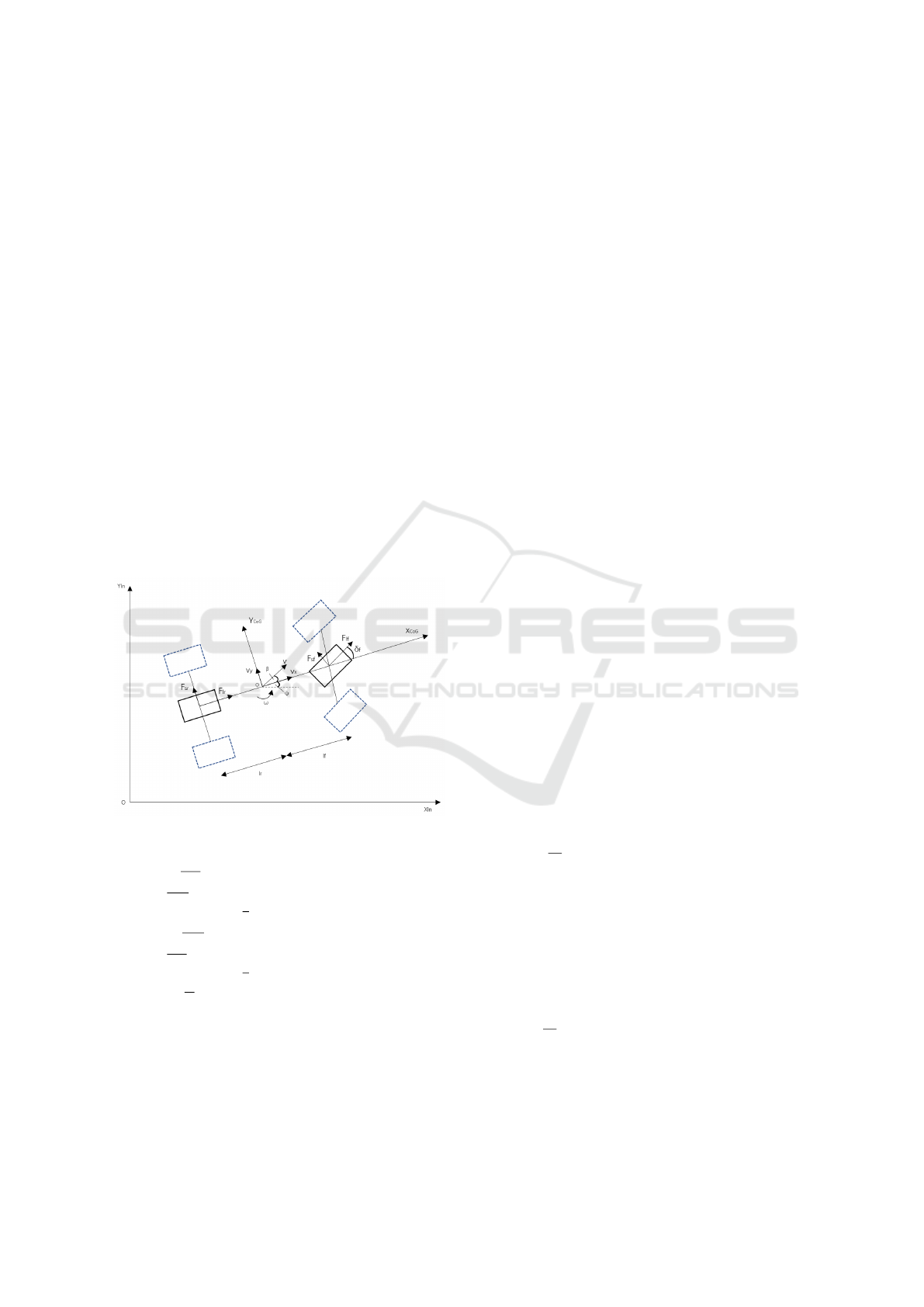
2.2 Vehicle Model
The dynamic model of the car is defined (Li, 2024).
In the simulation, this dynamic model is used to limit
the speed, angular speed and acceleration of the car.
The dynamic model of the car can be expressed by
Figure 1 and Equation 1:
Figure 1: Vehicle model.





















˙v =
sinβ
m
(F
s f
cosδ
f
+ F
l f
sinδ
f
+ F
s f
)
+
cosβ
m
(F
l f
cosδ
f
− F
s f
sinδ
f
+F
l f
−C
air
A
L
ρ
2
v
2
)
˙
β =
cosβ
mv
(F
s f
cosδ
f
+ F
l f
sinδ
f
+ F
s f
)
−
sinβ
mv
(F
l f
cosδ
f
− F
s f
sinδ
f
+F
l f
−C
air
A
L
ρ
2
v
2
)
˙
ω =
1
I
Z
(F
l f
l
f
sinδ
f
+ F
s f
l
f
cosδ
f
− F
sr
l
r
)
(1)
F
l f
, F
lr
are the longitudinal forces of the front and
rear wheels, respectively. F
s f
, F
sr
are the lateral forces
of the front and rear wheels, respectively. v, v
x
, v
y
are the vehicle speed, the longitudinal speed, and the
lateral speed. β, ψ, ω are the body side slip Angle,
the yaw Angle and the yaw speed. δ
f
is the steering
input Angle of the front wheel. l
f
is the distance from
center of gravity to front axle. l
r
is the distance from
center of gravity to the rear axis. m, I
Z
are the total
mass of the vehicle and yaw inertia, respectively. C
air
is the air drag coefficient. A
L
is the windward area. ρ
is the density of air.
The vehicle model will play a role in the later sim-
ulator validation section. Indicates that the planned
path given by the algorithm can be executed.
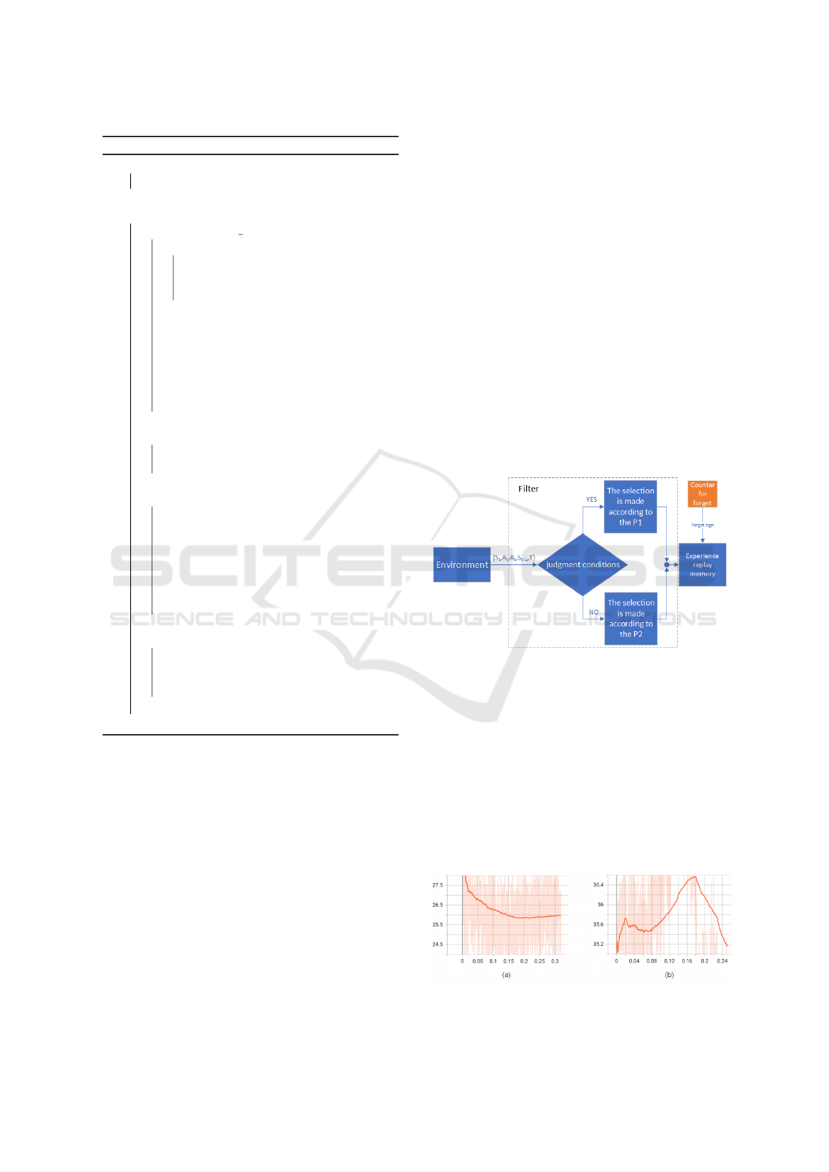
3 FILTER-FORGET MADDPG
3.1 Algorithm Flowchart and
Introduction
In this section, the FF-MADDPG diagram as given in
Algorithm 1:
θ
µ
and θ
Q
denote policy network and critic net-
work parameters in respect. τ is the soft update pa-
rameter.
Traditionally the MADDPG algorithm is a rein-
forcement learning algorithm used for multi-agent
systems, extending the DDPG algorithm from single-
agent environments. MADDPG allows multiple
agents to learn optimal strategies in cooperative or
competitive environments.
The algorithm consists of Critic networks with
their target networks and Actor networks with their
target networks. The Critic network provides a Q
function for each agent, evaluating a combination of
global state, actions of all agents, and the next state of
itself. The Actor network provides a policy for each
agent, directly reflecting the actions observed by the
agent.
The critic network is updated by the loss function,
as shown in Equation 2:
Loss =
1
M
∑
j
(q
i
− Q
µ
i
(x, a
1
, a
2
, a
3
, . . . , a
N
))
2
(2)
q
i
represents the target object Q value of the agent i ,
and its calculation formula is defined as Equation 3:
q
i
= r
i
+ γQ
µ
′
i
(x
′
, a
′
1
, a
′
2
, a
′
3
, . . . , a
′
N
) (3)
The actor network is subsequently updated by the
following policy gradient as shown in Equation 4:
∇
θ
i
J ≈
1
M
∑
j
∇
θ
i
µ
i
(s
i
)∇
a
i
Q
µ
i
(x, a
1
, a
2
, . . . , a
N
) (4)
MADDPG also includes an experience replay
buffer (run policies in the environment, collect the
state, action, reward, and next state for each agent).
Coordination for Complex Road Conditions at Unsignalized Intersections: A MADDPG Method with Enhanced Data Processing
295

Algorithm 1: FF-MADDPG in Each training time.
for agent i = 1 to N do
θ
µ
′
← θ
µ
, θ
Q
′
← θ
µ
end
while do
for t = 1 to max episode do
for agent i = 1 to N do
Obtain current environment state
s
t
. Select action a
t
according to
policy net, a
t
= µ(s
t
) + N
noise
.
end
Execute actions a
t
and calculate
reward r
t
as the formulas (8)
according to concrete situation and
acquire the new state s
t+1
. Through
the data filter,and store s
t
into
experience replay memory.
end
if Triggering the forget operation then
Delete previously stored data by
forgetting ratio.
end
for agent i = 1 to N do
Sample a random mini-batch samples
s
t
from experience replay memory.
Calculate Q value on the base of (3)
Update critic network by
minimizing the loss by (2) Update
actor network using the sampled
policy gradient by (4)
end
for agent i = 1 to N do
Update target network parameters by
θ
µ
′
← τθ
µ
+ (1 − τ)θ
µ
′
θ
Q
′
← τθ
Q
+ (1 − τ)θ
Q
′
end
end
Similar to DDPG, MADDPG uses an experience re-
play buffer to break the correlation of training data,
thus enhancing training stability.
However, due to the complexity of training en-
vironment, traditional methods are difficult to adapt.
Therefore, this paper improves upon the traditional
MADDPG approach to better adapt to experimental
environments.
There are two main changes:
Firstly, introducing a data filter: The bottlenecks
during learning in experiments caused a large amount
of collision data or extreme action data. These data
reduced the efficiency of data utilization. In order to
solve this problem, this paper designs a data filter. It
adjusts the proportions between various types of data
(such as collision data, extreme action data, normal
driving data) by setting a probability parameter to de-
termine whether to record the data.
Secondly, adopting phased forgetting for the data
pool: This paper introduces phased forgetting opera-
tion for the buffer, taking action to delete some data
when a certain amount is reached or when learning
bottlenecks are detected.
3.2 Contrast with Traditional Methods
The traditional method lacks the part of data process-
ing, including the storage and filtering of data. It just
stores all the data in the buffer and randomly extracts
it during training. As the amount of data continues
increasing, the information entropy of the extracted
data will significantly decrease, in other words, the
similarity of the data will be improved. This makes it
difficult for the neural network to learn more impor-
tant samples, resulting in a learning bottleneck prob-
lem.
Figure 2: Block diagram of the filter forgetting part.
Previously, the importance sample method has
been proposed, which adjusts the sampling probabil-
ity of some relatively important data. This method is
increases the efficiency by improving the learning in-
tensity of key information. The method proposed in
this paper is showed by Figure 2.
As the Figure 2 shows, data enters the buffer
through a filter. The input state through with differ-
ent probabilities depending on the conditions set. In
order to feel the benefits brought by this method more
intuitively, the 3AI1 human scene is used as the ex-
Figure 3: Information entropy comparison.
VEHITS 2025 - 11th International Conference on Vehicle Technology and Intelligent Transport Systems
296

Figure 4: Flowchart of algorithm.
perimental object to record its information entropy.
Histogram method was been used for the calculation
of information entropy.
The formula for information entropy is given by
Equation 5.

H(X) = −
∑
M
j
s
i j
log
2
s
i j
bins = 10
(5)
s
i j
denotes the jth bit of the state array of the ith
vehicle.
It is clear in Figure 3, The (a) is about the tradi-
tional approach, due to the continuous accumulation
of unfiltered data.
The operation of random fetching will increase the
probability of repeated data, as a result the informa-
tion entropy will be significantly reduced. The (b)
shows by data processing, the diversity of the data
within the buffer is ensured.
The flowchart of this paper’s algorithm is as
shown in Figure 4:
Q
µ
i
is denoted as the critic value in policy µ. Q
µ
′
i
is
denoted the target critic network. Superscript ′ de-
note the next time. a is denoted as the actions of
each agents. where N is the number of all agents,
and M is the number of mini-batch experiences ex-
tracted during training. x is the state of each agents
(s
1
, s
2
, s
3
, . . . , s
N
).
3.3 Constraints and Completion
Conditions
The vehicle motion constraints are specified as the ta-
ble 1:
Table 1: Vehicle constraints.
Variable Minimum value Maximum value
Path offset 0m 1m
Speed 0m/s 6m/s
Acceleration 0m/s
2
2m/s
2
X
o f f set
0m 2m
Y
o f f set
0m 2m
D
sa f e
5m +∞m
Schematic of the vehicle trajectory as shown in
Figure 5.
Figure 5: Path diagram.
The vehicle’s motion planning is mainly based on
a predetermined trajectory, At the same time, in order
Coordination for Complex Road Conditions at Unsignalized Intersections: A MADDPG Method with Enhanced Data Processing
297

to make the vehicle more skillfully deal with complex
road conditions, the vehicle is allowed to make some
degree of offset relative to the trajectory. X
o f f set
rep-
resents the offset on the X-axis relative to the planned
route. Y
o f f set
represents the offset on the Y-axis rela-
tive to the planned route. For the collision judgment
part, it is specified that within 5m from the vehicle
center point. Reaching the intersection where the plan
is reached is regarded as task completion. And D
sa f e
denotes the safe distance.
3.4 Parameter Setting
State is designed as shown in Equation 6:
s
i,t
= {P
sel f
, A
sel f
, P
other
, A
other
, D
other
, R
other
} (6)
s
i,t
denote the state space of the ith vehicle at time t.
P
sel f
is stand for the position of the car
i
, A
sel f
is stand
for the action of the car
i
, P
other
is stand for the posi-
tion of the other cars, A
other
is stand for the action of
the other cars, D
other
is stand for the distance between
the car
i
and other cars, A
other
is stand for the action
of the other cars. R
other
is stand for the relationship
between the car
i
and other cars. The relationship is as
shown in Equation 7:
R
other
=





−1, D
other
is smaller
0, D
other
is same
1, D
other
is bigger
(7)
The smaller, larger and the same in judgment condi-
tion, all compared to the D
other
at the time point be-
fore the moment.
Action is designed as shown in Equation 8:
a
i,t
= {X
o f f set
,Y
o f f set
, A
sel f
} (8)
a
i,t
denote the action space of the ith vehicle at
time t.
The reward function is designed State is designed
as shown in Equation 9:
r =









K
c
∗ (D
other
− D
sa f e
)
+K
a
∗ (A
sel f
), D
other
≤ D
sa f e
K
a
∗ (A
sel f
), D
other
>D
sa f e
(9)
K
c
,K
a
denotes the Gain coefficient.
Forgetting ratio: it refers to a certain proportion of
data forgetting work when a certain data capacity is
reached, see the flow chart
4 SIMULATION EXECUTION
4.1 Simulation Environment
In this paper, CARLA is used as the simulation plat-
form, the vehicle model in the experiment is ”Audi”,
and the control method is sliding mode control.
4.2 Design of Sliding-Mode Surface
Sliding Mode Control (SMC) is a nonlinear control
method, have strong robustness and fast response.
The method of sliding control was derived from
(Feng and Han, 2014). Define S
a
as the actual direc-
tion of the vehicle, S
t
as the target direction, x
1
as the
direction error, V
a
as the actual speed of the vehicle,
V
t
as the target speed, and x
2
as the speed error. T is
the throttle force of the vehicle and S is the steering
Angle of the steering wheel. t is the control time. k
1
,
k
2
, k
3
, k
4
are proportional coefficients.
The sliding-mode surface is designed as shown in
Equation 10:
s = k
1
T + k
2
sign(x
2
) | x
2
|
9
16
+k
3
x
9
23
1
(10)
Aiming at the problem of chattering in sliding mode
control, the control signal of throttle is designed as
shown in Equation 11:



u
eq
= −x
3
2
− k
2
sign(x
2
) | x
2
|
9
16
−k
3
x
9
23
1
u
n
= k
4
e
−t
+ 10 ∗ sign(s)
T = u
eq
+ u
n
(11)
The control signal of the steering wheel Angle is de-
rived from x
1
, k
5
is proportional coefficient and the
formula is as shown in Equation 12:
S = k
5
∗ x
1
(12)
5 RESULT AND DISCUSION
5.1 2AI and 1Human Situation
This scenario involves 2 AI vehicles and 1 human
driving vehicle.
Figure 6 shows the spatio-temporal relationship
diagram of the spatial locations of the three vehicles,
where the z-axis representing time and the X and Y
axes are the location coordinates of the intersection.
The red line (car 3) represents the human driving ve-
hicle, and the two figures show the perform of the AI
vehicle when the human driving vehicle is under dif-
ferent driving strategies. The results meet all previous
constraints and completion conditions.
VEHITS 2025 - 11th International Conference on Vehicle Technology and Intelligent Transport Systems
298

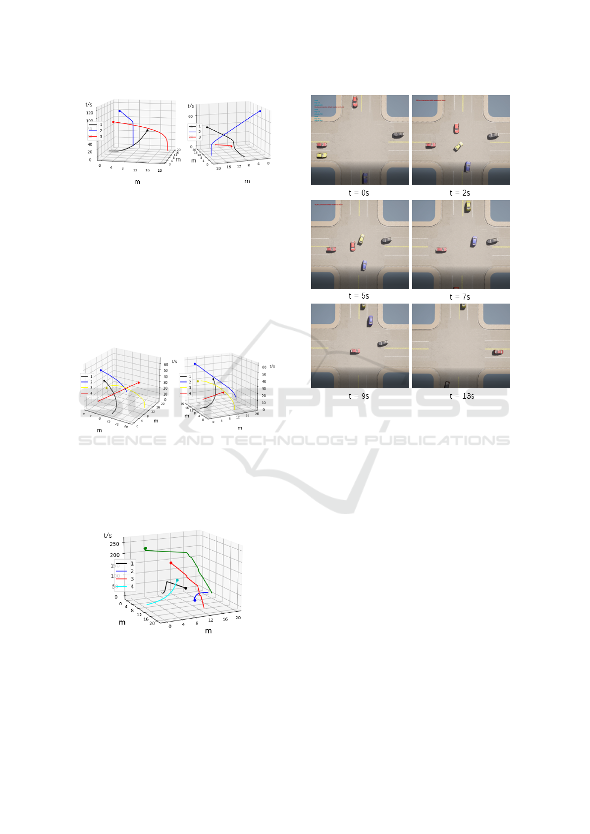
Figure 6: Trajectories in space–time of 2AI 1human.
5.2 3AI and 1Human Situation
This case is 3AI vehicles with one human driving ve-
hicle.
The Figure 7 shows the spatio-temporal relation-
ship diagram of the spatial position of the four cars.
The red line (car 4) represents the human driving ve-
hicle, and the two figures show the performance of
the AI vehicle when the human driving vehicle is un-
der different driving strategies. The results meet all
previous constraints and completion conditions.
Figure 7: Trajectories in space–time of 3AI 1human.
5 AI vehicles in this case.
The Figure 8 shows the spatio-temporal relation-
ship diagram of the spatial locations of the five ve-
hicles. The results meet all previous constraints and
completion conditions.
Figure 8: Trajectories in space–time of 5AI.
The result of CARLA can be seen from the Figure
9, at t=0s the car departs from the prescribed initial
point. Then the control strategy is executed accord-
ing to the speed and position plan given by the algo-
Figure 9: Simulation in CARLA.
rithm. At t=2s, t=5s, t=7s and t=9s, it can be clearly
seen that the autonomous vehicle responds to other
vehicles approaching for potential collisions. When
t=13s, it can be seen that the vehicles have completed
their assigned route and reached their respective des-
tinations.
6 CONCLUSIONS
In this paper, an improved MADDPG algorithm is
proposed and applied to solve the intersection plan-
ning problem of autonomous vehicles and human ve-
hicles. The effectiveness of the algorithm is verified
using sliding mode control in CARLA.
The main contributions of this paper are as fol-
lows:
(1) A more effective MADDPG algorithm for data
processing is proposed to address the issue of deep re-
inforcement learning frequently encountering bottle-
necks in complex environments.
(2) A reinforcement learning framework is built to
handle the intersection scene with involving human
driving vehicles, so that the autonomous driving ve-
Coordination for Complex Road Conditions at Unsignalized Intersections: A MADDPG Method with Enhanced Data Processing
299

hicle can not only deal with the full AI-controlled en-
vironment but also handle the complex environment
with human driving vehicles.
ACKNOWLEDGEMENT
This work is supported by Zhejiang Provincial
Natural Science Foundation of China (Grant No.
LQ23F030014), National Natural Science Foundation
of China (Grant No. 62303410), and Open Research
Project of State Key Laboratory of Industrial Control
Technology, Zhejiang University, China (Grant No.
ICT2024B46).
REFERENCES
Chen, C. and Xu, Q. (2022). Conflict-free coopera-
tion method for connected and automated vehicles
at unsignalized intersections: Graph-based modeling
and optimality analysis. IEEE Transactions on Intel-
ligent Transportation Systems, 23(11):21897–21914.
Feng, Y. and Han, F. (2014). Chattering free full-order
sliding-mode control. Automatica, 50(4):1310–1314.
Feng, Y. and Head, K. L. (2015). A real-time adaptive signal
control in a connected vehicle environment. Trans-
portation Research Part C: Emerging Technologies,
55:460–473.
Li, A. (2024). Intelligent Vehicle Perception, Trajectory
Planning and Control. Chemical Industry Press, Bei-
jing, 1 edition.
Li, L. and Wang, F. (2006). Cooperative driving at blind
crossings using intervehicle communication. IEEE
Transactions on Vehicular Technology, 55(6):1712–
1724.
Lowe, R., Wu, Y., Tamar, A., Harb, J., Abbeel, P., and Mor-
datch, I. (2020). Multi-agent actor-critic for mixed
cooperative-competitive environments.
Malikopoulos, A. A. and Cassandras, C. G. (2018). A
decentralized energy-optimal control framework for
connected automated vehicles at signal-free intersec-
tions. Automatica, 93:244–256.
Shirazi, M. S. and Morris, B. T. (2017). Looking at intersec-
tions: A survey of intersection monitoring, behavior
and safety analysis of recent studies. IEEE Transac-
tions on Intelligent Transportation Systems, 18(1):4–
24.
Shobana, S. and Shakunthala, M. (2023). Iot based on smart
traffic lights and streetlight system. In 2023 2nd Inter-
national Conference on Edge Computing and Appli-
cations (ICECAA), pages 1311–1316.
Wang, B. and Gong, X. (2024). Coordination for con-
nected and autonomous vehicles at unsignalized in-
tersections: An iterative learning-based collision-free
motion planning method. IEEE Internet of Things
Journal, 11(3):5439–5454.
Wu, Y. and Chen, H. (2019). Dcl-aim: Decentralized coor-
dination learning of autonomous intersection manage-
ment for connected and automated vehicles. Trans-
portation Research Part C: Emerging Technologies,
103:246–260.
Xu, H. and Zhang, Y. (2020). Cooperative driving at
unsignalized intersections using tree search. IEEE
Transactions on Intelligent Transportation Systems,
21(11):4563–4571.
Xu, J. and Liu, C. (2024). Resource allocation in multi-uav
communication networks using maddpg framework
with double reward and task decomposition. pages
371–376.
Zhang, J. and Ge, J. (2024). A bi-level network-wide coop-
erative driving approach including deep reinforcement
learning-based routing. IEEE Transactions on Intelli-
gent Vehicles, 9(1):1243–1259.
Zhang, J. and Li, S. (2023). Coordinating cav swarms
at intersections with a deep learning model. IEEE
Transactions on Intelligent Transportation Systems,
24(6):6280–6291.
Zhou, J. and Zhu, F. (2020). Modeling the fundamental
diagram of mixed human-driven and connected au-
tomated vehicles. Transportation Research Part C:
Emerging Technologies, 115:102614.
VEHITS 2025 - 11th International Conference on Vehicle Technology and Intelligent Transport Systems
300