Centralised Urban Traffic Routing Using Mixed-Integer Programming
Andrii Nyporko
1,2 a
, Maty
´
a
ˇ
s
ˇ
Svadlenka
1,2 b
, Nikolai Antonov
1,2 c
,
Mohammad Rohaninejad
1 d
and Luk
´
a
ˇ
s Chrpa
1 e
1
Czech Institute of Informatics, Robotics and Cybernetics, Czech Technical University in Prague, Czechia
2
Faculty of Electrical Engineering, Czech Technical University in Prague, Czechia
Keywords:
Centralised Traffic Routing, Mixed-Integer Programming, Urban Traffic Management.
Abstract:
The increase in the urban population over the past decades led to an increase in the number of vehicles in urban
road networks, especially in larger metropolitan areas. The problem is exacerbated during rush hours and when
an unexpected or rare event occurs (e.g. accidents, concerts). Existing traffic routing methods, including those
embedded in modern navigation systems, consider Dynamic User Optimal (DUO) traffic routing that generates
routes in a decentralised fashion. Centralized traffic routing, which we consider in this paper, benefits from the
global perspective of the situation that can utilise the road network more effectively. We propose a technique
leveraging Mixed-Integer Programming (MIP) for distributing vehicles in the road network while minimizing
traffic intensity on road segments. Our evaluation shows the potential of the proposed technique for centralized
traffic routing.
1 INTRODUCTION
Over the past decades, the urban population has been
steadily increasing. That contributed to an increase
in traffic intensity in urban areas, especially during
rush hours. Traffic congestion is one of the major
economic problems as, for example, the cost of con-
gestion in London exceeded £5 billion in 2020
1
. On
top of that, heavy traffic in urban areas poses a major
health threat (Chang et al., 2019). Occasional events,
such as sports matches, rallies, or concerts, also have
a major impact on urban traffic that might be more
difficult to predict.
The concept of Smart Cities (Kirimtat et al., 2020)
involves the need for effective traffic management,
focusing on the proper distribution of traffic in road
networks to minimize average travel time and dis-
tance traveled. In addition to initiatives such as
car sharing to reduce the number of vehicles, ef-
fective traffic management utilizes road infrastruc-
ture through efficient traffic routing and traffic light
a
https://orcid.org/0000-0001-5535-4250
b
https://orcid.org/0009-0004-9199-3024
c
https://orcid.org/0009-0002-0156-3561
d
https://orcid.org/0000-0002-0623-4890
e
https://orcid.org/0000-0001-9713-7748
1
https://www.london.gov.uk/press-releases/mayoral/
cost-of-congestion-in-capital-revealed
control, which has been approached from a cen-
tralized perspective through scheduling (Xie et al.,
2012), evolutionary methods (Pil
´
at, 2018), and au-
tomated planning (Pozanco et al., 2021; McCluskey
and Vallati, 2017; Antoniou et al., 2019). These
strategies are incorporated into a framework that in-
troduces pheromone-based traffic management (Cao
et al., 2017). Modern navigation systems, such as
those employing the Dynamic User Optimal (DUO)
principle (Friesz et al., 1989), generate optimal routes
in a decentralized manner by leveraging current traf-
fic data. However, decentralized routing can cause is-
sues, such as unsynchronised routing to network bot-
tlenecks.
Centralized traffic routing aims to provide the op-
timal route for each vehicle from a global perspec-
tive of the controlled region, thereby utilizing the road
network more effectively. In more detail, centralised
traffic routing has to involve centralised infrastructure
to vehicle (I2V, V2I) communication such that vehi-
cles approaching the controlled region must broad-
cast their entry and exit points, allowing the infras-
tructure to generate routes, for all the vehicles ap-
proaching the region in a given time span, that are
then broadcast back to the vehicles. Approaches in
centralized traffic routing involve collecting data on
vehicles’ intended routes, predicting future traffic in-
tensity, and broadcasting this prediction back to vehi-
176
Nyporko, A., Švadlenka, M., Antonov, N., Rohaninejad, M. and Chrpa, L.
Centralised Urban Traffic Routing Using Mixed-Integer Programming.
DOI: 10.5220/0013137100003890
Paper published under CC license (CC BY-NC-ND 4.0)
In Proceedings of the 17th International Conference on Agents and Artificial Intelligence (ICAART 2025) - Volume 2, pages 176-187
ISBN: 978-989-758-737-5; ISSN: 2184-433X
Proceedings Copyright © 2025 by SCITEPRESS – Science and Technology Publications, Lda.

cles for route updates. Recent methods focus on us-
ing automated planning for centralized dynamic route
allocation (Chrpa et al., 2019; Vallati et al., 2021;
Svadlenka et al., 2023; Silva and Tang, 2024).
Current automated planning based techniques for
centralised traffic routing reason on the individual ve-
hicle level while computing routes (Chrpa et al., 2019;
Svadlenka et al., 2023). Even though we need to com-
pute the route for each individual vehicle, it is impor-
tant to optimise traffic flows first (i.e., determine how
many vehicles use which route) as this information is
crucial to determine expected traffic intensity on par-
ticular road segments. Thus, the decision about traffic
flows does not have to be made on the “microsimu-
lation” level (the individual vehicle level) as it is cur-
rently done in the planning-based methods.
Hence, in this paper, we focus on the “microsim-
ulation” aspect of planning-based centralized traffic
routing such that we introduce a Mixed-Integer Pro-
gramming (MIP) model (Wolsey, 1998), inspired by
the multicomodity network flow problem (Ouorou
et al., 2000), that distributes traffic across the road
network, aiming to minimize traffic intensity on road
segments. In contrast to planning-based techniques,
we consider macrosimulation that, in other words,
distribute traffic at the “flow” level. The main advan-
tage of the proposed approach is that routes do not
have to be recomputed multiple times and that many
symmetries can be broken (e.g. the order in which
vehicles are routed). To extract routes for individual
vehicles, we propose an algorithm, based on Depth-
First-Search, that searches through the allocated traf-
fic flows (the solution of the MIP model).
Our approach was evaluated on scenarios from
New York and Sydney metropolitan areas (Svadlenka
et al., 2023) as well as on a central region of
Dublin (Gueriau and Dusparic, 2020) by using the
well-known SUMO simulator (Lopez et al., 2018).
The results show the potential of our approach as it
outperforms the decentralised (DUO) as well as the
existing planning-based approaches for Centralised
Traffic Routing in the New York and Sydney scenar-
ios. We provide a thorough analysis of the results,
discuss the limitations of the current approach as well
as the lessons we learned, and provide some ideas for
improvements that we plan to address in future work.
2 RELATED WORKS
The concept of Smart Cities (Kirimtat et al., 2020) in-
corporates the need for effective traffic management
involving a proper distribution of traffic in road net-
works, minimising average travel time and average
driven distance. Besides initiatives that aim at re-
ducing the number of vehicles (e.g. by car-sharing),
effective traffic management has to utilize road in-
frastructure through effective traffic routing and ef-
fective traffic light control. Both traffic optimisa-
tion strategies are considered in a framework that in-
troduced pheromone-based traffic management (Cao
et al., 2017). Traffic light control has been tackled
from a centralised perspective by means of schedul-
ing (Xie et al., 2012), evolutionary approaches (Pil
´
at,
2018), or automated planning (Pozanco et al., 2021;
McCluskey and Vallati, 2017; Antoniou et al., 2019).
Traffic routing methods that are embedded in mod-
ern navigation systems (e.g. WAZE™) usually follow
the Dynamic User Optimal (DUO) principle (Friesz
et al., 1989) that, in a nutshell, generates (optimal)
routes in a decentralised fashion while leveraging cur-
rent traffic data (Du et al., 2014; Claes et al., 2011). A
possible issue of decentralised (DUO) routing might
involve unsynchronised routing to “network bottle-
necks” that might not (yet) be busy when routing
takes place.
The centralised traffic routing approaches, on the
other hand, aim to provide the optimal route for each
vehicle from the global perspective of the (controlled)
region and hence can utilise the controlled road net-
work more effectively. Each vehicle approaching the
controlled region has to broadcast its intentions, i.e.,
where it enters the network and where it plans to leave
the network. The infrastructure that collects the in-
formation from approaching vehicles has to provide
routes for the vehicles across the controlled region.
Yamashita et al. (Yamashita et al., 2005) proposed an
approach that collects data about vehicles’ intended
routes, based on the collected data it makes a predic-
tion of future traffic intensity in the area, and the pre-
diction is broadcasted back to vehicles, so the vehicles
might update their routes according to the prediction.
Recent Centralised Traffic Routing approaches are
mostly based on Automated Planning (Chrpa et al.,
2019; Vallati et al., 2021; Svadlenka et al., 2023) and,
most recently, on centralised dynamic route alloca-
tion (Silva and Tang, 2024).
Although planning-based approaches achieved
promising results (Chrpa et al., 2019; Svadlenka et al.,
2023), they tend to struggle with scalability and might
be suitable only for smaller regions (Chrpa and Val-
lati, 2023). The size of the road network in which
centralised traffic routing techniques have to reason
in can be reduced by precomputing suitable routes for
each traffic flow (Svadlenka et al., 2023; Silva and
Tang, 2024). Another aspect contributing to the poor
scalability of centralised traffic routing techniques is
the need to provide a route for each individual vehicle,
Centralised Urban Traffic Routing Using Mixed-Integer Programming
177

i.e., considering microsimulation.
There are approaches addressing the vehicle rout-
ing problem, which optimizes routes to serve cus-
tomers, usually by minimising the total travel dis-
tance, or mitigating possible delays. This draws a
parallel with our work, although the goals are differ-
ent – optimising traffic flows in traffic routing versus
optimising delivery services. One of the most recent
approaches (Polimeni and Vitetta, 2024) proposed an
approach tackling the problem of integrating road net-
work design and vehicle routing (public and freight
transport). Also, we can pinpoint (Wenning et al.,
2006) and (Krishnan et al., 2017), where this problem
is tackled in decentralised fashion that draws some
parallel between decentralised and centralised traffic
routing.
3 CENTRALISED TRAFFIC
ROUTING
In a nutshell, the problem of Centralised Traffic Rout-
ing can be understood as finding routes for a set of
vehicles in a road network, where each vehicle has
its locations of origin and destination while optimis-
ing for specified criteria such as minimising aver-
age travel time or minimising traffic intensity on the
road segments. In this paper, we use the concept
of Centralised Traffic Routing described by Chrpa et
al. (Chrpa et al., 2019).
3.1 Problem Specification
Formally, the Centralised Traffic Routing problem is
a tuple χ = (N ,V, O, D,C), where N represent a road
network in form of a labeled directed graph N =
(N, E, R, ρ), where vertices N represent junctions and
edges E connect the adjacent junctions by road seg-
ments from R by a mapping ρ : E → R. Note that we
admit that more edges can be mapped to a single road
segment (because of the representation of road net-
works in SUMO and simplifications we applied such
as “merging” roundabouts into a single junction). Let
V = {v
1
, . . . , v
k
} be a set of vehicles that approach the
network such that each vehicle has its location (junc-
tion) of origin, specified by a function O : V → N, and
its destination location (junction), specified by a func-
tion D : V → N. Note that a pair (origin,destination)
refers to a traffic flow. A function C : R × N
0
→ R
+
0
represents the cost for using a road segment by a given
number of vehicles.
We say that Σ = {p
1
, . . . , p
k
} is a solution of χ if
and only if for each i ∈ {1, . . . , k} it is the case that p
i
is a sequence of edges from E forming a path in N
starting at O(v
i
) and finishing at D(v
i
). The cost of Σ
is determined as
∑
x∈R
C(x, |{i | e ∈ p
i
, x = ρ(e)}|).
We would like to note that the cost of navigating
through junctions (e.g. traffic lights) is relaxed out.
A Centralised Traffic Routing problem is gener-
ated according to the current traffic situation period-
ically, i.e., every n seconds, as proposed in (Chrpa
et al., 2019; Svadlenka et al., 2023). In particular, ve-
hicles’ intentions, i.e., where they enter the controlled
region and where they leave the region, are collected
for vehicles that are approaching the region. Gener-
ated routes are then assigned to the vehicles (before
they enter the region). Automated planning-based ap-
proaches, in a nutshell, tackle the problem by con-
sidering “drive” actions, specifying the “elementary”
moves of vehicles between adjacent junctions using
a corresponding road segment (Chrpa et al., 2019;
Svadlenka et al., 2023). In practice, vehicles collect
information with their sensors about traffic status and
transmit this information and their intentions to the
centralised system. This information is used to gen-
erate data for solving the problem of distributing the
traffic in the system - creating/updating the paths, and
finally assigning them to each vehicle.
3.2 Determining Cost Through Traffic
Intensity
Each road segment has its capacity, i.e., the maxi-
mum theoretical number of vehicles that can fit into
the segment while also considering a minimum space
between vehicles. If the number of vehicles routed
to the given road segment exceeds its capacity, then
we say that the road segment is congested. Then we
specify two thresholds that divide the traffic inten-
sity into (additional) three levels – light, medium and
heavy. To draw a parallel between the categories and
the well-known Level of Service, the light intensity
level corresponds to grades A and B, the medium in-
tensity level to C and D, and the heavy intensity level
to E and F. Such a categorization has also been pro-
posed in (Chrpa et al., 2019; Svadlenka et al., 2023).
The cost of the road segment is then determined
by its length, its number of vehicles, and its traffic in-
tensity category. Since we distinguish four categories
of traffic intensity, i.e., light, medium, heavy, con-
gested, we define for each road segment r ∈ R thresh-
olds u
l
r
, u
m
r
, u
h
r
determining the maximum number of
vehicles for the light, medium, and heavy traffic in-
tensity level, respectively, and constants l
r
, m
r
, h
r
,C
r
representing the cost of a single vehicle for respective
traffic intensity level.
Then, the cost function is a piecewise linear func-
tion as follows.
ICAART 2025 - 17th International Conference on Agents and Artificial Intelligence
178

C(r, n) = n · l
r
(n ∈ [0, u
l
r
]), n · m
r
(n ∈ (u
l
r
, u
m
r
]),
n · h
r
(n ∈ (u
m
r
, u
h
r
]), n ·C
r
(n ∈ (u
h
r
, ∞))
(1)
3.3 Road Network Simplification
Automated-planning-based centralised traffic routing
techniques reason on the level of individual vehicles,
i.e., on the micro-simulation level. Therefore, the size
of the road network in which these techniques reason
is one of the considerable factors that affect their per-
formance as the route has to be computed for each
individual vehicle (Chrpa and Vallati, 2023).
A straightforward way how to simplify the road
network is to precompute routes for each traffic flow
that have bounded suboptimality (Svadlenka et al.,
2023; Silva and Tang, 2024). Arguably, long routes
might not be very efficient even in light traffic. Such
routes with bounded suboptimality can be found by an
algorithm combining Floyd-Warshall algorithm with
Branch and Bound algorithm (Silva and Tang, 2024)
or by a variant of A* with the Euclidean-distance
heuristic (Svadlenka et al., 2023). The latter approach
is considered in our experiments.
Further reduction of the size of the network to
reason with can be done by precomputing “smart”
routes that besides being bounded suboptimal are di-
verse enough so they might not share “common bot-
tlenecks” (Svadlenka et al., 2023). In particular,
bounded suboptimal routes are clustered according to
the Jaccard Index by which the diversity of routes
(based on comparing sets of their road segments) is
determined and then, from each cluster, one route
is selected (e.g. the shortest one) (Svadlenka et al.,
2023).
Note that even though our MIP model works on
the level of traffic flows, i.e., macro-simulation, we
can still leverage the above simplification methods.
4 CENTRALISED TRAFFIC
ROUTING MIP MODEL
The proposed MIP model draws inspiration from mul-
ticommodity flow problems (Ouorou et al., 2000),
which are the type of network flow problem (Ahuja
et al., 1993) with multiple commodities. Multicom-
modity flow problem is a fundamental class of op-
timization problems, often forming the backbone of
other more intricate applications in telecommunica-
tions, logistics, and transportation (Fortz et al., 2017).
Our MIP model goes beyond traditional multicom-
modity flow formulations for urban traffic systems,
as the routing cost functions are continuous, convex,
and piecewise linear. These cost functions are well-
suited for capturing the different levels of urban traffic
flow. This incorporation is particularly time-sensitive
in centralised traffic routing, requiring real-time plan-
ning due to the dynamic environment. Therefore, we
restricted our approach to a tight optimization time,
which is well-designed for dynamic environments. To
the best of our knowledge, this work is the first to
integrate network flows with multiple commodities
for centralized (urban) traffic routing while offering
a novel perspective on real-time traffic flow routing in
metropolitan environments.
4.1 Multiflow MIP Model
We aim at optimizing multicommodity flows to mini-
mize traffic intensity on road segments while ensuring
that vehicles entering a junction also leave it, main-
taining flow integrity. A single traffic flow, defined
by a specific origin and destination, is restricted to
a subgraph of the road network created through pre-
processing methods. We identify the number of ve-
hicles that have to be routed in the considered traffic
flow. For the junction of origin/destination, the sum
of outgoing/incoming traffic flow equals to the num-
ber of routed vehicles. For any other junction, the
flow conservation law holds, i.e. the sum of incoming
traffic flow equals the sum of outgoing one. Decision
variables for traffic intensity in each flow are modeled
separately to maintain consistency and ensure all ve-
hicles reach their destinations. While different flows
can share road segments, the traffic intensity and cost
on each segment depend on the total traffic from all
flows using that segment.
Given the Centralised Traffic Routing problem
χ = (N ,V, O, D,C), the initial step is to identify traf-
fic flows. Each traffic flow is represented by a pair
of (origin,destination) junctions in which vehicles (of
that traffic flow) enter and leave the region, respec-
tively. A traffic flow i is represented by a triple
(o
i
, d
i
, n
i
), where o
i
, d
i
∈ N are origin and destina-
tion junctions of i, respectively, and n
i
= |{v | v ∈
V, O(v) = o
i
, D(v) = d
i
}| is the number of vehicles in
the flow i. We consider only traffic flows that are not
empty, i.e., there is at least one vehicle in them. The
number of non-empty traffic flows (of χ) is denoted
as N
F
. A subset of edges that might be generated by
any preprocessing technique that simplifies the road
network (as described in Section 3.3) for the flow i is
denoted as E
i
(E
i
⊆ E).
The above idea of leveraging the concept of net-
work flows for routing traffic (in each flow separately)
is modelled as follows. We introduce x variables
Centralised Urban Traffic Routing Using Mixed-Integer Programming
179

representing the number of vehicles of a given flow
routed on a given edge, i.e., x
i
u,v
represents the num-
ber of vehicles of flow i routed on edge (u, v) ∈ E
i
.
Then for each non-empty traffic flow i ∈ {1, ..., N
F
},
we define the following equations.
∀(u, v) ∈ E : x
i
u,v
∈ N
0
,
∑
w∈V,(o
i
,w)∈E
i
x
i
o
i
,w
=
∑
(w,d
i
)∈E
i
x
i
w,d
i
(2)
∑
(o
i
,w)∈E
i
x
i
O,w
= n
i
(3)
∑
(v,o
i
)∈E
i
x
i
v,o
i
= 0 (4)
∑
(d
i
,w)∈E
i
x
i
d
i
,w
= 0 (5)
∑
(u,v)∈E
i
,u̸=o
i
x
i
u,v
=
∑
(v,w)∈E
i
,w̸=d
i
x
i
v,w
(6)
∀(u, v) ∈ E \ E
i
: x
i
u,v
= 0 (7)
Equation (2) represents that the sum of all outgo-
ing subflows from the origin junction equals the sum
of all incoming subflows into the destination junction.
Equation (3) determines the number of vehicles in the
flow. Equations (4) and (5) ensure that none of the
vehicles in the flow can return to the origin junction
as well as no vehicle can reenter the network from
the destination junction. Equation (6) represents that
for all junctions, other than origin and destination, the
sum of all incoming traffic must be equal to the sum
of outgoing traffic. The x
i
variables defined on edges
that are not part of E
i
are set to 0 (Equation (7)).
The objective function that we want to optimise
in our model minimises the cost of the allocation of
traffic flows in the road network. The original opti-
mization equation, presented in Section 3.2 makes our
model quadratic, so, in order to tackle that as solvers
handle linear models more effectively, we will repre-
sent that equation in a linearised form as our model
objective function, i.e.:
min
∑
r∈R
y
r
Note that the cost of traffic allocation on an edge de-
pends on the number of vehicles in it and that mul-
tiple edges might share a single corresponding road
segment.
One common approach involves linearising piece-
wise functions, where distinct regions defined by bi-
nary variables cause nonlinearity. Concerning that,
we will formulate the equation (1) so that the cost for
each edge and each traffic level is calculated as fol-
lows:
y
r
≥ l
r
N
F
∑
i=1
∑
(u,v)
r=ρ((u,v))
x
i
u,v
− M(1 − z
l
r
) (8)
y
r
≥ m
r
N
F
∑
i=1
∑
(u,v)
r=ρ((u,v))
x
i
u,v
− M(1 − z
m
r
) (9)
y
r
≥ h
r
N
F
∑
i=1
∑
(u,v)
r=ρ((u,v))
x
i
u,v
− M(1 − z
h
r
) (10)
y
r
≥ C
r
N
F
∑
i=1
∑
(u,v)
r=ρ((u,v))
x
i
u,v
− M(1 − z
C
r
) (11)
In the presented model the cost of two junctions is cal-
culated by a piecewise function (1) where the binary
variables z
l
r
, z
m
r
, z
h
r
, and z
C
r
are used (light, medium,
heavy, congested, respectively), each representing a
region of the piecewise function and determining the
level of traffic intensity on the road segment r accord-
ing to the number of vehicles allocated on it. By
imposing constraints that link these binary variables
to the objective function through linear inequalities,
the nonlinear objective function can be obtained with
a series of linear segments (constraints (8) to (11)).
Note that M is a (very) big constant, the usage of
which combined with the constraint (12) ensures that
only one segment (traffic intensity level) is active at
a time, effectively capturing the behavior of the orig-
inal nonlinear objective function. The model showed
the best performance with M equal to 10 million after
testing it with different values.
∀r ∈ R
z
l
r
∈ {0; 1}, z
m
r
∈ {0; 1}, z
h
r
∈ {0; 1}, z
C
r
∈ {0; 1}
z
l
r
+ z
m
r
+ z
h
r
+ z
C
r
= 1 (12)
N
F
∑
i=1
∑
(u,v)
r=ρ((u,v))
x
i
u,v
≤ z
l
r
u
l
r
+ z
m
r
u
m
r
+ z
h
r
u
h
r
+ z
C
r
M (13)
N
F
∑
i=1
∑
(u,v)
r=ρ((u,v))
x
i
u,v
≥ z
m
r
u
l
r
+ z
h
r
u
m
r
+ z
C
r
u
h
r
(14)
Equation (12) represents that only one traffic in-
tensity level can be chosen for a given road segment.
Equations (13) and (14) represent the upper and lower
bounds for the number of vehicles (from all flows)
for the respective traffic intensity level. The thresh-
olds u
l
r
, u
m
r
, u
h
r
represent the maximum number of ve-
hicles on the road segment r that can be considered
as a light, medium, or heavy level of traffic intensity,
ICAART 2025 - 17th International Conference on Agents and Artificial Intelligence
180

respectively. The model successfully works without
the equation (14), but it helps with the continuous re-
laxation of the model, enhancing the performance and
computational speed.
4.2 Extracting Routes for Vehicles
The solution of the MIP model provides informa-
tion on how particular traffic flows are distributed in
the road network. Specifically, the decision variables
x contain information about the number of vehicles
from a given traffic flow allocated to a given road seg-
ment. Such information is however insufficient as we
need to know the exact routes for all the vehicles.
Algorithm 1 describes the procedure of extracting
routes alongside the number of vehicles allocated to
each of the routes for a single traffic flow. Therefore,
the algorithm is called for each traffic flow separately.
As an input, the algorithm takes a description of the
road network, the solution of the MIP model, the iden-
tifier of the given traffic flow (i), and its starting junc-
tion (the location of origin).
The algorithm performs a Depth First Search
while looking for individual routes, which is imple-
mented by recursively calling the SearchRoute func-
tion. The current (partial) route is stored in p and the
current junction in j.
We initially look for outgoing edges from j (in the
road network graph) that have some vehicles allocated
to them, i.e., the value of x
i
for a given edge is greater
than zero (Line 2). If none such outgoing edge exists,
then we reached the destination ( j is the destination
location since there was an incoming traffic to j but
there is no outgoing traffic). We extract the route p
and the number of vehicles (veh count) for p equals
the minimum of allocated vehicles per each edge on
the route p (additional traffic on some edges belongs
to other routes). Then, we decrement the values of
x on the route by veh count. If some outgoing edge
from j is already in p, then we have a loop (Line 10).
We might encounter loops if the MIP solver returns a
suboptimal solution that might happen, for example,
if we impose time limits on the solver. If a loop is
identified, we remove it by decrementing the x val-
ues on the loop by the minimum of these x values
(Lines 12–13). In other situations, we iterate through
the outgoing edges (with some traffic on them) such
that we append the edge to p and call the SearchRoute
with a subsequent junction (Lines 15–18).
We can see that the algorithm performs an exhaus-
tive Depth First Search such that it only follows edges
(road segments) that have some traffic allocated to
them. Since the sum of outgoing traffic for a junc-
tion (other than the origin or destination) equals the
Function SearchRoute(p, j, i, all routes):
outgoing edges = {( j, j
′
) | ( j, j
′
) ∈
E, x
i
j, j
′
> 0};
if outgoing edges =
/
0 then
; /* We extracted a route */
veh count ← min
( j
x
, j
y
)∈p
x
i
j
x
, j
y
;
if veh count> 0 then
all routes ←
all routes∪{(p, veh count)};
∀( j
x
, j
y
) ∈ p : x
i
j
x
, j
y
← x
i
j
x
, j
y
−
veh count;
end
else
if ∃( j, j
′
) ∈ p then
; /* We found a loop */
p
j
← p.subpath from( j);
veh count ← min
( j
x
, j
y
)∈p
j
x
i
j
x
, j
y
;
∀( j
x
, j
y
) ∈ p
j
: x
i
j
x
, j
y
← x
i
j
x
, j
y
−
veh count;
else
for (j, j
′
) ∈ outgoing edges do
p.append(( j, j
′
));
SearchRoute(p, j
′
, i,
all routes);
end
end
end
SearchRoute(⟨⟩, start junction, i, {});
Algorithm 1: Algorithm for extracting routes for a given
traffic flow.
sum of incoming traffic, there always exists an outgo-
ing edge that has some traffic allocated to it (unless
we are in the destination junction). We have two sit-
uations in which we stop searching in a given branch
(and then backtrack and continue searching another
branch until we explore all the branches). Firstly, we
reach the destination junction. In such a way we can
extract the route (from the origin) and the amount of
traffic equals the minimum of the current allocation
on the edges of the route. Updating the traffic allo-
cation then reflects the extracted route and the traf-
fic on it. The second “stopping” situation concerns
loop detection (that might happen if the solution of
the MIP model is suboptimal). We then identify the
amount of traffic in the loop and update the traffic al-
location by removing the traffic that is on that loop. It
should be noted that loop detection (and elimination)
improves the quality of the MIP solution since the re-
sulting routes do not contain loops (albeit the MIP so-
lution does). Since we perform an exhaustive search,
we eventually extract routes that cover all routed vehi-
Centralised Urban Traffic Routing Using Mixed-Integer Programming
181

cles. Note that decisions made during the search, i.e.,
the order in which the successors are explored might
affect resulting routes (and traffic allocation on them).
In other words, the solution of the MIP model might
yield multiple valid routing solutions.
The final step, after Algorithm 1 finishes for every
traffic flow, is to allocate extracted routes to the ve-
hicles. For each traffic flow, we select vehicles that
belong to this traffic flow and then we iterate over
all routes (from Algorithm 1) and, in an iteration step,
we assign the current route to the respective number
of (yet unallocated) vehicles. We would like to note
that there might not be a single unique route alloca-
tion for the vehicles if the number of routes is greater
than one. In our case, we allocate routes in the or-
der they are stored in all routes to vehicles ordered by
their ids.
5 EXPERIMENTAL EVALUATION
The aim of the experimental evaluation is to show the
potential of our MIP-based technique for Centralised
Traffic Routing. In particular, we compare against
a planning-based technique that uses “smart route”
preprocessing (Svadlenka et al., 2023) to show that
our macrosimulation-based MIP approach is more
scalable and capable of more effective traffic rout-
ing than microsimulation-based planning approaches.
On top of that, we also compare against the decen-
tralised (DUO) approach for dynamic traffic rout-
ing that is implemented within the SUMO simula-
tor (Lopez et al., 2018).
The quality of routing is measured by the average
travel time that is extracted from the simulation (by
SUMO). To provide a bigger picture, we also mea-
sured the average traveled distance and the average
speed. Note that SUMO simulations consider aspects
that we relaxed out (e.g. traffic lights). Simulations
concerning Centralised Traffic Routing are done of-
fline, i.e., vehicles routes are computed in advance.
5.1 Scenarios and Settings
For the experiments, we used two scenarios - New
York (located between Grand Concourse and Sheri-
dan Boulevard) and Sydney (southeast of Centen-
nial Park) - that were introduced by Svadlenka et
al. (Svadlenka et al., 2023) (depicted in Figure 1).
For New York and Sydney, we have considered 16
and 40 scenarios, respectively, that differ by traffic
flows (origin and destination) and how flows evolve in
time (static or increasing). For all scenarios, we con-
sidered a 1-hour time window that was divided into
30-second “episodes” where each corresponded to a
single instance of a Centralised Traffic Routing prob-
lem. Hence, for each scenario, we considered 120
episodes. For New York, we considered 5 traffic flows
per scenario while for Syndey 4 traffic flows per sce-
nario. The traffic intensity ranged between 760 and
1208 vehicles per hour per traffic flow. The simula-
tion of (routed) traffic ran for 2 hours in SUMO. The
road network, in both cases, is initially empty and the
first vehicles arrive into the network at time zero (of
the simulation time).
Additionally, we considered a scenario from
central Dublin, where we used a real historical
dataset (Gueriau and Dusparic, 2020). The central re-
gion was selected according to the most intense traf-
fic (depicted in orange in Figure 2). We considered
an almost 2-hour time window spanning from 7am to
9am (the morning rush hour). Again, we divided the
time window into 30-second episodes, yielding 238
episodes in total. The total number of routed vehicles
was 10 778. The simulation of (routed) traffic also
ran for 2 hours in SUMO. The road network, again,
is initially empty and the first vehicles arrive into the
network at time zero (of the simulation time).
As described in Section 3.3, we preprocessed the
original road network in two ways. One involves
generating bounded suboptimal routes for each traf-
fic flow (the bound was set to 1.3 as in (Svadlenka
et al., 2023)), which we later denote as BR. The
other “smart routes” preprocessing method involves
clustering of potential routes based on their di-
versity (i.e., having fewer road segments in com-
mon) and selecting the shortest route for each clus-
ter (Svadlenka et al., 2023). This preprocessing
method is later denoted as SR. Both BR and SR pre-
processing methods are used with MIP method as
well as with the planning method we compare against
(for which the preprocessing methods were originally
designed) (Svadlenka et al., 2023).
The thresholds determining the level of traffic in-
tensity for road segments are derived from the physi-
cal capacity of the road segment that is measured by
the number of “standard” vehicles that can physically
fit into the road segment while considering a mini-
mum distance between them. Light traffic intensity of
a road segment corresponds to the number of routed
vehicles up to 40% of its capacity. Medium traffic in-
tensity of a road segment corresponds to the number
of routed vehicles from 40% to 60% of its capacity.
Heavy traffic intensity of a road segment corresponds
to the number of routed vehicles higher than 60%
of its capacity but not more than the capacity. Con-
gested traffic intensity of a road segment corresponds
to the number of routed vehicles higher than its ca-
ICAART 2025 - 17th International Conference on Agents and Artificial Intelligence
182

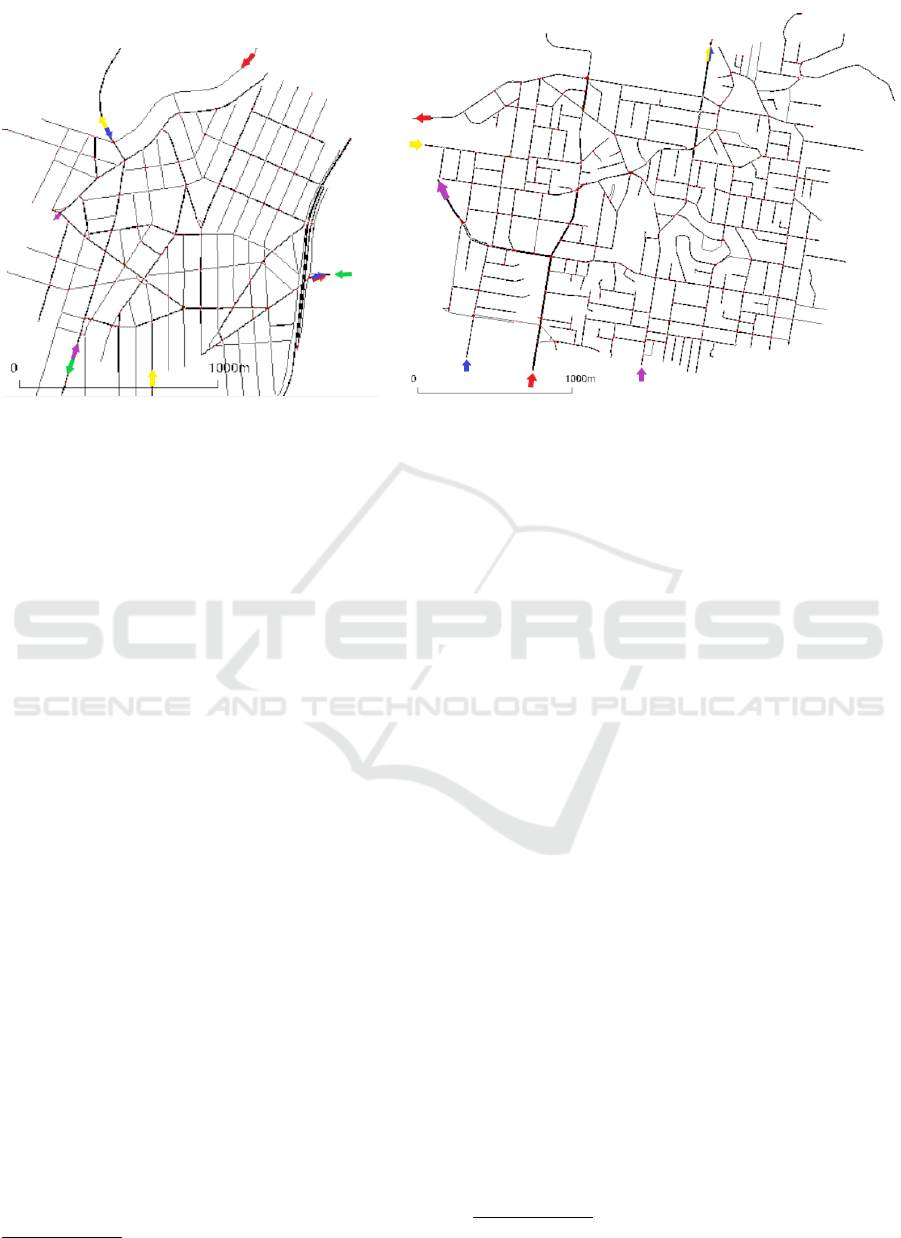
(a) New York region (b) Sydney region
Figure 1: The New York (left) and Sydney (right) scenarios. The colored arrows illustrate sample traffic flows (their entry and
exit points to the controlled area). The scenarios are taken from (Svadlenka et al., 2023).
pacity. These thresholds are determined in analogy
with (Vallati et al., 2021). The cost of a road segment
(for a single vehicle) with light traffic intensity equals
the length of the road segment. The cost of a road
segment (for a single vehicle) with medium traffic in-
tensity equals 10 times the length of the road segment.
The cost of a road segment (for a single vehicle) with
heavy traffic intensity equals 100 times the length of
the road segment. The cost of a road segment (for a
single vehicle) with congested traffic intensity equals
100000. Note that the cost is determined in analogy
to (Chrpa et al., 2019; Svadlenka et al., 2023).
For solving the MIP model, the global nonlinear
solver Gurobi was also chosen for his ability to work
with quadratic models
2
. Since we need to obtain the
solution within a certain time limit (one episode con-
siders 30 seconds of traffic), process it, and send it
back, the runtime is limited to 25 seconds. For the
planning-based approach, we use the Mercury plan-
ner (Domshlak et al., 2015) with a time limit of 25
seconds as well. In case we fail to find any solution
for a given episode within the time limit, we assign
the shortest routes (for New York and Sydney), or the
routes specified in the historical dataset (for Dublin)
for all the vehicles considered in the failed planning
episode.
In a nutshell, we have extracted the following met-
rics from simulating the different routing methods in
SUMO (Lopez et al., 2018). Average trip distance,
i.e., how many meters the vehicles had to travel on av-
erage, average trip duration, i.e., how many seconds
2
https://www.gurobi.com/documentation/
the vehicles had to take to reach their destinations,
and average speed (in meters per second). The exper-
iments were run on a computer equipped with AMD
Ryzen 5000 7, with a memory limit of 32GB
3
.
5.2 Results
The results of the experiments are summarised in Ta-
ble 1. Noteworthy, for New York and Sydney, the re-
sults are averaged for all considered scenarios with
different traffic flows (16 for New York and 40 for
Sydney). It can be seen that in all scenarios and
both variants of pre-processing optimisations of the
road network (BR and SR), MIP approach solves (not
necessarily optimally) all episodes (instances of the
Centralised Traffic Routing problem). Compared to
the planning approach, MIP model has shown that
it is capable of scaling (much) better, which is espe-
cially apparent for the BR cases (where we consider
bounded sub-optimal routes for each traffic flow)
where the planning approaches solved (not necessar-
ily optimally) only a few episodes.
Focusing on the average trip duration, which is
the metric we optimise for, in contrast to planning,
MIP achieved better results for the BR preprocessing.
Whereas in planning, the SR preprocessing, which
pre-computes several promising routes for each traf-
fic flow, is essential for improving the coverage (i.e.,
the percentages of solved episodes), for MIP model
SR is too restrictive and introduces suboptimality (as
3
Benchmark data are provided here: https://github.com/
xankr/utc-mip-icaart2025
Centralised Urban Traffic Routing Using Mixed-Integer Programming
183

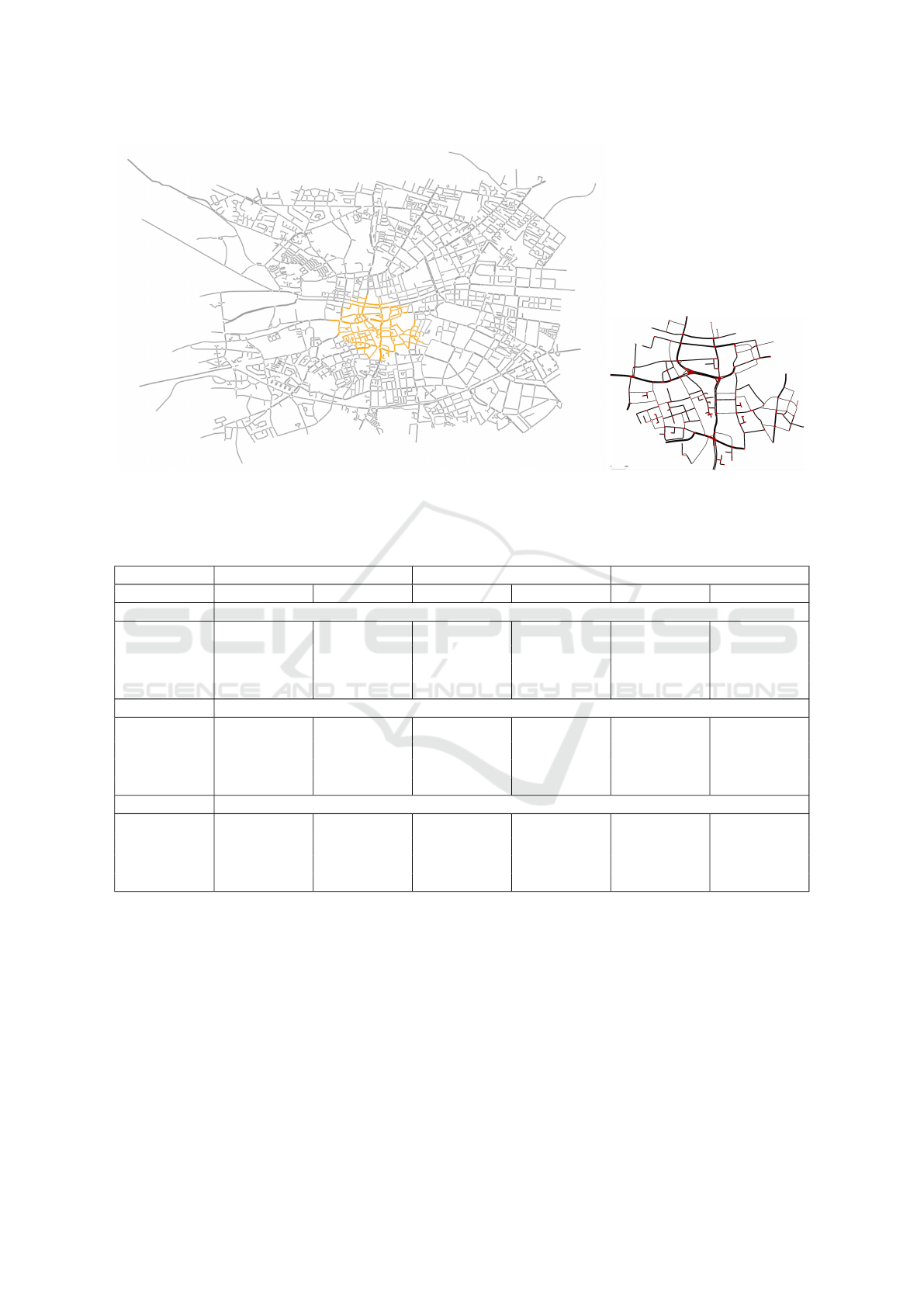
Figure 2: Image of the whole Dublin metropolitan area (left) and the considered city center scenario (right)
Table 1: Simulation results for all city benchmarks. “Solved” denotes the percentage of solved episodes (not necessarily
optimally) by the MIP and Planning approaches. “Distance”, “Speed” and “Duration” denote the average trip distance,
average speed, and average trip duration, respectively.
Parameters Baseline MIP Planning
Naive DUO BR SR BR SR
New York
Solved [%] - - 100 100 9.1 74.5
Distance [m] 1915 2355 2385 2136 2042 2361
Speed [m/s] 1.95 2.76 3.18 2.69 2.26 3.07
Duration [s] 1670 1356 1193 1388 1605 1235
Sydney
Solved [%] - - 100 100 1.77 46.9
Distance [m] 2608 2980 3002 2901 2454 2770
Speed [m/s] 3.38 5.6 6.74 5.75 3.35 3.86
Duration [s] 1324 746 641 761 1245 1160
Dublin
Solved [%] - - 100 100 0 96.6
Distance [m] 828 904 812 822 828 835
Speed [m/s] 5.13 6.15 5.92 5.52 5.13 5.81
Duration [s] 360 229 276 283 360 226
can be seen from the results for MIP). Comparing the
best results (of average trip duration) between MIP
and planning, we can see that in Sydney the MIP-
based approach is better by about 45%, in New York
slightly better (about 4%), while in Dublin, it is worse
by about 20%. In comparison to the Naive approach
that, in the New York and Sydney scenarios, consid-
ers shortest routes, the MIP approach improves the
average trip duration by about 30% and more than
50%, respectively. In Dublin, where the Naive ap-
proach consists of historical traffic data (hence the
routes are not necessarily the shortest), the improve-
ment of the MIP-based approach was roughly 25%.
Concerning DUO, the MIP-based approaches outper-
formed it in New York and Sydney by roughly 12%
and 14%, respectively, while in Dublin, they were
worse by about 17%. Interestingly, in the Dublin sce-
nario, the planning approach (with the SR preprocess-
ing) was slightly better than DUO. To provide a better
perspective we compared the best approach in each
category in Figure 3.
In terms of average trip distance, it is no surprise
that all routing approaches tend to generate longer
routes in order to mitigate traffic intensity on exposed
ICAART 2025 - 17th International Conference on Agents and Artificial Intelligence
184

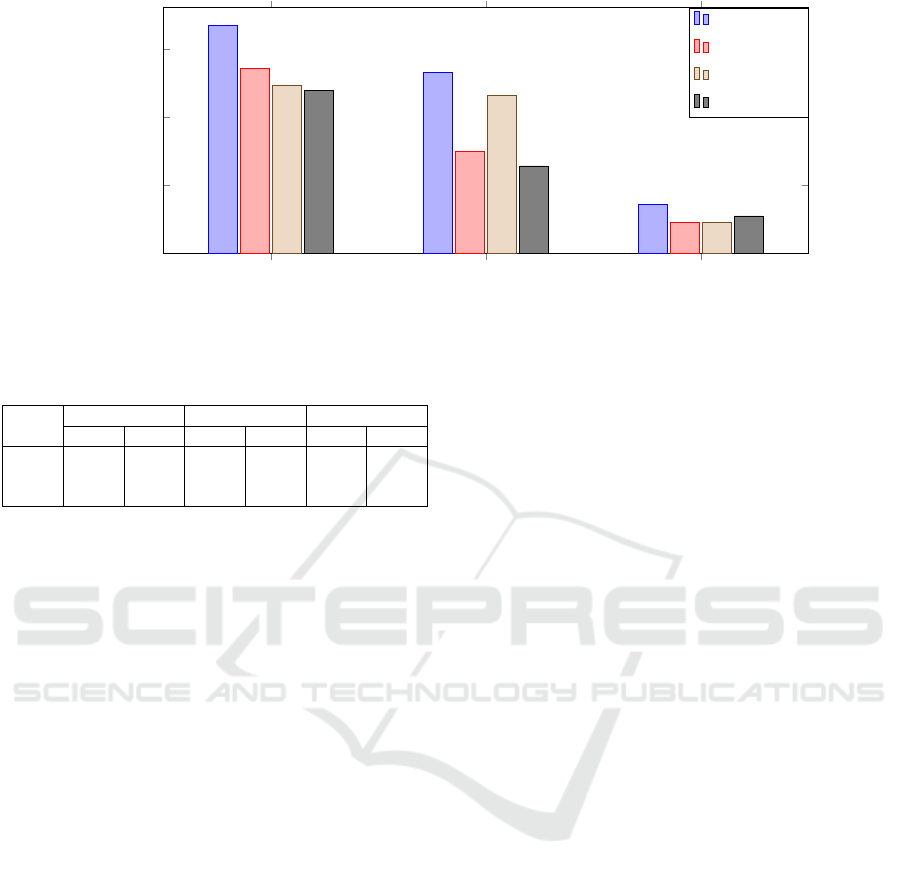
New York Sydney Dublin
0
500
1,000
1,500
Duration [s]
Naive
DUO
Planning SR
MIP BR
Figure 3: Average Trip Duration Comparison for Different Methods per Scenario.
Table 2: Average total runtime (PT [s]), average number of
optimally solved scenarios (OPT [%]) and average optimal-
ity gap (GAP [%]) of MIP.
New York Sydney Dublin
BR SR BR SR BR SR
PT 328 62 247 45 1005 452
OPT 100 100 99.8 100 97.1 100
GAP 0 0 0.95 0 2.8 0
road segments. In the New York scenario, the routes
get more than 20% longer in comparison to the Naive
approach. On the other hand, the average speed in-
creased by more than 50% which not only compen-
sated for longer driven distance but also saved some
time. In the Dublin scenario, the average trip distance
for all centralised routing approaches is roughly the
same as in the Naive approach, yet it leads to better
trip duration results (note that the planning results for
BR are the same as Naive as none of the episodes was
solved). DUO, on the other hand, had longer routes
by about 10%, which led to better utilisation of the
road network (measured by the average speed).
5.3 Discussion
The results have shown that leveraging MIP-based
techniques is a viable option for dealing with Cen-
tralised Traffic Routing problems as these techniques
provide better scalability than techniques based on
automated planning. That said, the macrosimulation
type of reasoning on the level traffic (sub)flows alle-
viates some symmetries that are associated with the
microsimulation type of reasoning since there is no
difference in terms of the objective function which in-
dividual vehicle takes which route. For example, if v
1
takes route r
1
and v
2
takes r
2
(assuming that v
1
and v
2
belong to the same traffic flow), the value of our ob-
jective function will be the same as if v
2
takes r
1
and
v
1
takes r
2
.
Better performance of the MIP approach led to im-
provement of the overall results, measured by the av-
erage trip duration, in New York and Sydney, outper-
forming all the other methods. In Dublin, however,
MIP underperformed both DUO and the planning ap-
proaches. The main difference between the New York
and Sydney scenarios and the Dublin scenario is that
in the former we deal with several traffic flows (5 and
4, respectively) each with several vehicles (at most
20) per episode, while in Dublin, the number of traffic
flows is larger often containing a single vehicle (in a
single episode). This aspect mitigates the benefits of
macrosimulation as for “single-vehicle” flows there
is no difference to microsimulation. The reason for
“scattered” traffic flows in Dublin is that most vehi-
cles start or finish their trip within the region.
Another aspect that affects the results is the ac-
curacy of the objective function, i.e., how it reflects
the actual traffic situation. As Table 2 summarises,
the MIP approach generated optimal solutions in most
cases and almost optimal in the rest. The objective
function we use in this paper has been specified in
the literature (Chrpa et al., 2019; Vallati et al., 2021;
Svadlenka et al., 2023) with the rationale to reduce
traffic intensity for the road segments in the con-
trolled (urban) region. The objective function, how-
ever, might not accurately capture some nuances such
as the shape of road segments and, more importantly,
how the segments are connected. For example, if traf-
fic from a side road is merging with the traffic on a
main road on an uncontrolled junction, it might in-
troduce additional bottlenecks as the traffic from the
side road might not (easily) merge if the traffic on
the main road is (slightly) more intense. We have
observed such situations in the simulations that had
a detrimental impact on the results. Also, in con-
trast to DUO, our objective function does not consider
the current traffic situation outside the given planning
episode (e.g., while routing we do not get informa-
tion about heavy traffic that is currently on some road
segments).
Centralised Urban Traffic Routing Using Mixed-Integer Programming
185

The lessons we have learned indicate that Cen-
tralised Traffic Routing (via MIP) is a viable way
to effectively route traffic in urban regions suffering
from heavy traffic (especially in rush hours). De-
spite the above drawbacks, the results have shown that
our MIP method can outperform the decentralised ap-
proaches (DUO) in scenarios in which we route sev-
eral more intense traffic flows (such as in the New
York and Sydney scenarios). In other words, Cen-
tralised Traffic Routing seems to work effectively in
scenarios in which we route transit traffic from mul-
tiple traffic flows that might interfere with each other.
We believe that centralised traffic routing can com-
plement the decentralised one as we might identify
common traffic flows (that interfere with each other)
and route only vehicles in these flows by centralised
routing techniques while the other vehicles by decen-
tralised routing techniques.
6 CONCLUSION
In this paper, we have addressed the Centralised Traf-
fic Routing problem by means of Mixed-Integer Pro-
gramming by modelling the problem as a combination
of multiple network flows. We designed a MIP model
that naturally captures the cost function (as specified
in the literature (Chrpa et al., 2019; Svadlenka et al.,
2023)). We have shown that the macrosimulation
level reasoning that MIP allows improves scalabil-
ity over the microsimulation-based approaches such
as those based on automated planning (Chrpa et al.,
2019; Svadlenka et al., 2023). In terms of Centralised
Traffic Routing in general, our experiments (espe-
cially those on the New York and Sydney scenarios)
showed that it has a good potential to outperform dis-
tributed routing methods that are nowadays routinely
exploited in navigation systems. The lessons learned
from the experiments indicate that Centralised Traffic
Routing has more potential in routing several more in-
tense traffic flows rather than a large number of “scat-
tered” traffic flows (as happened in the Dublin sce-
nario).
In the future, we plan to investigate how effec-
tively we can identify bottlenecks (e.g. merging from
the side road on an uncontrolled junction) and how
these bottlenecks can be effectively represented in the
objective function. Also, we plan to investigate how
we can effectively identify “common traffic flows” in
larger urban areas and how to integrate Centralised
Traffic Routing techniques on these flows into other
(decentralised) routing approaches.
ACKNOWLEDGMENTS
This research is supported by Czech Science Founda-
tion (project no. 23-05575S), by the European Union
under the OP JAK project ROBOPROX (reg. no.
CZ.02.01.01/00/22 008/0004590), and by the Grant
Agency of the Czech Technical University (project
no. SGS24/115/OHK3/2T/37).
REFERENCES
Ahuja, R. K., Magnanti, T. L., and Orlin, J. B. (1993).
Network flows: theory, algorithms, and applications.
Prentice-Hall, Inc., USA.
Antoniou, G., Batsakis, S., Davies, J., Duke, A., Mc-
Cluskey, T. L., Peytchev, E., Tachmazidis, I., and Val-
lati, M. (2019). Enabling the use of a planning agent
for urban traffic management via enriched and inte-
grated urban data. Transportation Research Part C:
Emerging Technologies, 98:284 – 297.
Cao, Z., Jiang, S., Zhang, J., and Guo, H. (2017). A unified
framework for vehicle rerouting and traffic light con-
trol to reduce traffic congestion. IEEE Transactions on
Intelligent Transportation Systems, 18(7):1958–1973.
Chang, K.-H., Hsu, P.-Y., Lin, C.-J., Lin, C.-L., Juo,
S.-H. H., and Liang, C.-L. (2019). Traffic-related
air pollutants increase the risk for age-related macu-
lar degeneration. Journal of Investigative Medicine,
67(7):1076–1081.
Chrpa, L. and Vallati, M. (2023). Centralised vehicle rout-
ing for optimising urban traffic: A scalability per-
spective. In IEEE Intelligent Vehicles Symposium, IV
2023, Anchorage, AK, USA, June 4-7, 2023, pages 1–
6. IEEE.
Chrpa, L., Vallati, M., and Parkinson, S. (2019). Exploit-
ing automated planning for efficient centralized vehi-
cle routing and mitigating congestion in urban road
networks. In Proceedings of the 34th ACM/SIGAPP
Symposium on Applied Computing, SAC 2019.
Claes, R., Holvoet, T., and Weyns, D. (2011). A decentral-
ized approach for anticipatory vehicle routing using
delegate multiagent systems. IEEE Transactions on
Intelligent Transportation Systems, 12(2):364–373.
Domshlak, C., Hoffmann, J., and Katz, M. (2015). Red-
black planning: A new systematic approach to partial
delete relaxation. Artif. Intell., 221:73–114.
Du, L., Han, L., and Li, X.-Y. (2014). Distributed coordi-
nated in-vehicle online routing using mixed-strategy
congestion game. Transportation Research Part B:
Methodological, 67:1–17.
Fortz, B., Gouveia, L., and Joyce-Moniz, M. (2017). Mod-
els for the piecewise linear unsplittable multicommod-
ity flow problems. European Journal of Operational
Research, 261(1):30–42.
Friesz, T. L., Luque, J., Tobin, R. L., and Wie, B.-W. (1989).
Dynamic network traffic assignment considered as a
continuous time optimal control problem. Operations
Research, 37(6):893–901.
ICAART 2025 - 17th International Conference on Agents and Artificial Intelligence
186

Gueriau, M. and Dusparic, I. (2020). Quantifying the im-
pact of connected and autonomous vehicles on traffic
efficiency and safety in mixed traffic. In 23rd IEEE In-
ternational Conference on Intelligent Transportation
Systems.
Kirimtat, A., Krejcar, O., Kertesz, A., and Tasgetiren, M. F.
(2020). Future trends and current state of smart city
concepts: A survey. IEEE Access, 8:86448–86467.
Krishnan, A., Markov, M., and Bonakdarpour, B. (2017).
Distributed vehicle routing approximation. In 2017
IEEE International Parallel and Distributed Process-
ing Symposium (IPDPS), pages 503–512.
Lopez, P. A., Behrisch, M., Bieker-Walz, L., Erdmann, J.,
Fl
¨
otter
¨
od, Y.-P., Hilbrich, R., L
¨
ucken, L., Rummel, J.,
Wagner, P., and Wießner, E. (2018). Microscopic traf-
fic simulation using sumo. In Proceedings of ITSC.
McCluskey, T. L. and Vallati, M. (2017). Embedding auto-
mated planning within urban traffic management op-
erations. In Proceedings of the Twenty-Seventh In-
ternational Conference on Automated Planning and
Scheduling, ICAPS 2017, pages 391–399.
Ouorou, A., Mahey, P., and Vial, J.-P. (2000). A survey
of algorithms for convex multicommodity flow prob-
lems. Management science, 46(1):126–147.
Pil
´
at, M. (2018). Evolving ensembles of traffic lights con-
trollers. In IEEE 30th International Conference on
Tools with Artificial Intelligence, ICTAI 2018, pages
958–962. IEEE.
Polimeni, A. and Vitetta, A. (2024). Network design and ve-
hicle routing problems in road transport systems: In-
tegrating models and algorithms. Transportation En-
gineering, 16:100247.
Pozanco, A., Fern
´
andez, S., and Borrajo, D. (2021). On-
line modelling and planning for urban traffic control.
Expert Systems.
Silva, M. D. R. L. and Tang, M. (2024). A new frame-
work for centralized coordinated multi-vehicle dy-
namic routing. IEEE Access, 12:24243–24253.
Svadlenka, M., Chrpa, L., and Vallati, M. (2023). Improv-
ing the scalability of automated planning-based vehi-
cle routing via smart routes identification. In 8th In-
ternational Conference on Models and Technologies
for Intelligent Transportation Systems, MT-ITS 2023,
pages 1–6. IEEE.
Vallati, M., Scala, E., and Chrpa, L. (2021). A hybrid au-
tomated planning approach for urban real-time rout-
ing of connected vehicles. In 24th IEEE International
Intelligent Transportation Systems Conference, ITSC,
pages 3821–3826. IEEE.
Wenning, B.-L., Timm-Giel, A., and Pesch, D. (2006). A
distributed routing approach for vehicle routing in lo-
gistic networks. In IEEE Vehicular Technology Con-
ference, pages 1 – 5.
Wolsey, L. A. (1998 - 1998). Integer programming / Lau-
rence A. Wolsey. Wiley-Interscience series in discrete
mathematics and optimization. J. Wiley, New York.
Xie, X.-F., Smith, S., and Barlow, G. (2012). Schedule-
driven coordination for real-time traffic network con-
trol. In Proceedings of ICAPS.
Yamashita, T., Izumi, K., Kurumatani, K., and Nakashima,
H. (2005). Smooth traffic flow with a cooperative car
navigation system. In 4th International Joint Confer-
ence on Autonomous Agents and Multiagent Systems
(AAMAS 2005), pages 478–485. ACM.
Centralised Urban Traffic Routing Using Mixed-Integer Programming
187